Lab 6

Author

Affiliation

Filippo Gambarota

University of Padova

devtools::load_all()
library(tidyverse)
library(ggeffects)
library(here)

Overview

EDA

Loading data

load(here("data", "psych.rda"))
dat <- psych

Given that we did not introduced random-effects models, we select a single subject to analyze.

cc <- seq(0, 1, 0.1)

dat$contrast_c <- cut(dat$contrast, cc, include.lowest = TRUE)

dat |> 
  filter(id %in% sample(unique(dat$id), 5)) |> 
  group_by(id, cond, contrast_c) |> 
  summarise(y = mean(y)) |> 
  ggplot(aes(x = contrast_c, y = y, color = cond, group = cond)) +
  geom_point() +
  geom_line() +
  theme(axis.text.x = element_text(angle = 90)) +
  facet_wrap(~id)

`summarise()` has grouped output by 'id', 'cond'. You can override using the
`.groups` argument.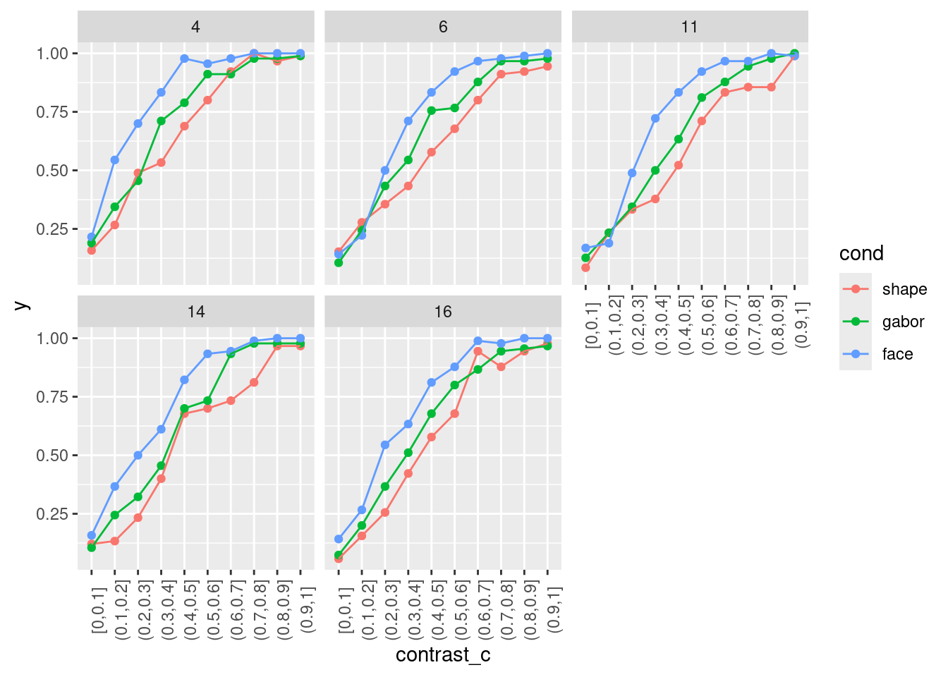

dat <- filter(dat, id == 6)

We have several interesting stuff to estimate. Let’s start by fitting a simple model:

fit1 <- glm(y ~ contrast, data = dat, family = binomial(link = "logit"))
summary(fit1)

Call:
glm(formula = y ~ contrast, family = binomial(link = "logit"), 
    data = dat)

Coefficients:
            Estimate Std. Error z value Pr(>|z|)    
(Intercept) -1.97038    0.08949  -22.02   <2e-16 ***
contrast     6.25920    0.21843   28.66   <2e-16 ***
---
Signif. codes:  0 '***' 0.001 '**' 0.01 '*' 0.05 '.' 0.1 ' ' 1

(Dispersion parameter for binomial family taken to be 1)

    Null deviance: 4007.1  on 2999  degrees of freedom
Residual deviance: 2531.5  on 2998  degrees of freedom
AIC: 2535.5

Number of Fisher Scoring iterations: 5

The parameters (Intercept) and contrast are respectively the probability of saying yes for stimuli with 0 contrast. Seems odd but in Psychophysics this is a very interesting information. We can call it the false alarm rate. We usually expect this rate to be low, ideally 0.

plogis(coef(fit1)[1])

(Intercept) 
  0.1223485 

The contrast is the slope i.e. the increase in the log odds of saying yes for a unit increase in contrast. In this case this parameter is hard to intepret, let’s change the scale of the contrast:

dat$contrast10 <- dat$contrast * 10
fit1 <- glm(y ~ contrast10, data = dat, family = binomial(link = "logit"))
summary(fit1)

Call:
glm(formula = y ~ contrast10, family = binomial(link = "logit"), 
    data = dat)

Coefficients:
            Estimate Std. Error z value Pr(>|z|)    
(Intercept) -1.97038    0.08949  -22.02   <2e-16 ***
contrast10   0.62592    0.02184   28.66   <2e-16 ***
---
Signif. codes:  0 '***' 0.001 '**' 0.01 '*' 0.05 '.' 0.1 ' ' 1

(Dispersion parameter for binomial family taken to be 1)

    Null deviance: 4007.1  on 2999  degrees of freedom
Residual deviance: 2531.5  on 2998  degrees of freedom
AIC: 2535.5

Number of Fisher Scoring iterations: 5

Now the contrast10 is the increase in the log odds of saying yes for an increase of 10% contrast. Using the divide-by-4 rule we obtain an maximal increase of 0.15648 of probability of saying yes.

Another interesting parameter is the threshold. In psychophysics the threshold is the required \(x\) level (in this case contrast) to obtain a certain proportions of \(y\) response.

For a logistic distribution [see @Knoblauch2012-to] the 50% threshold can be estimated as \(-\frac{\beta_0}{\beta_1}\) thus:

-(coef(fit1)[1]/coef(fit1)[2])

(Intercept) 
   3.147967 

Then the slope is simply the inverse of the regression slope and represent the increase in performance/visibility for a unit increase in \(x\):

1/coef(fit1)[2]

contrast10 
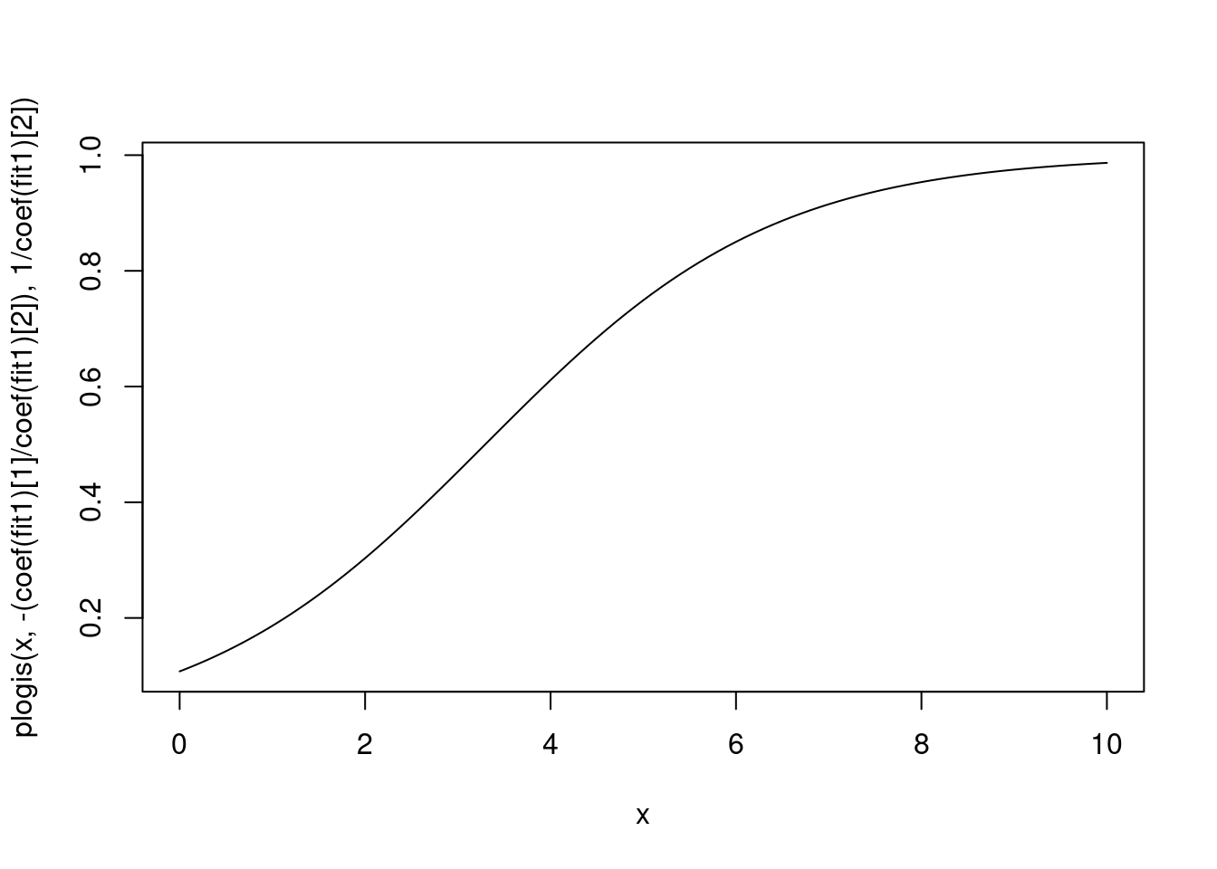
  1.597648 

In fact, we can use these parameters to plot a logistic distribution:

curve(plogis(x, -(coef(fit1)[1]/coef(fit1)[2]), 1/coef(fit1)[2]),
      0, 10)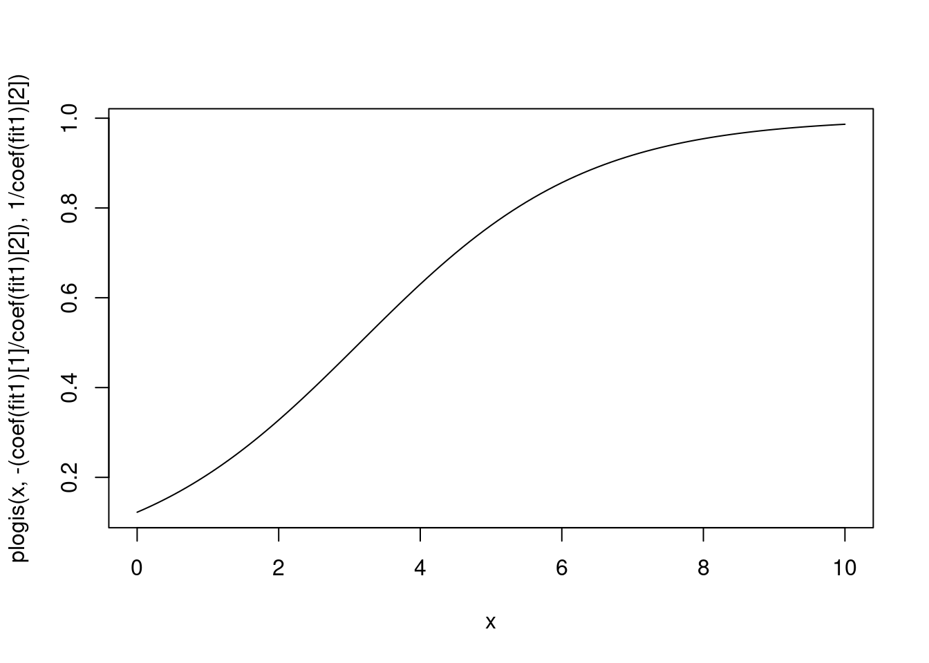

That is very similar to the effects estimated by our model:

plot(ggeffect(fit1))

References