
N <- 200
b0 <- 0.2
b1 <- 2
s <- 1

x <- runif(N, 0, 1)
y <- rnorm(N, b0 + b1 * x, s)

data.frame(x, y) |>
    ggplot(aes(x = x, y = y)) +
    geom_point(size = 3) +
    geom_smooth(method = "lm", se = FALSE, formula = y ~ x, lwd = 2)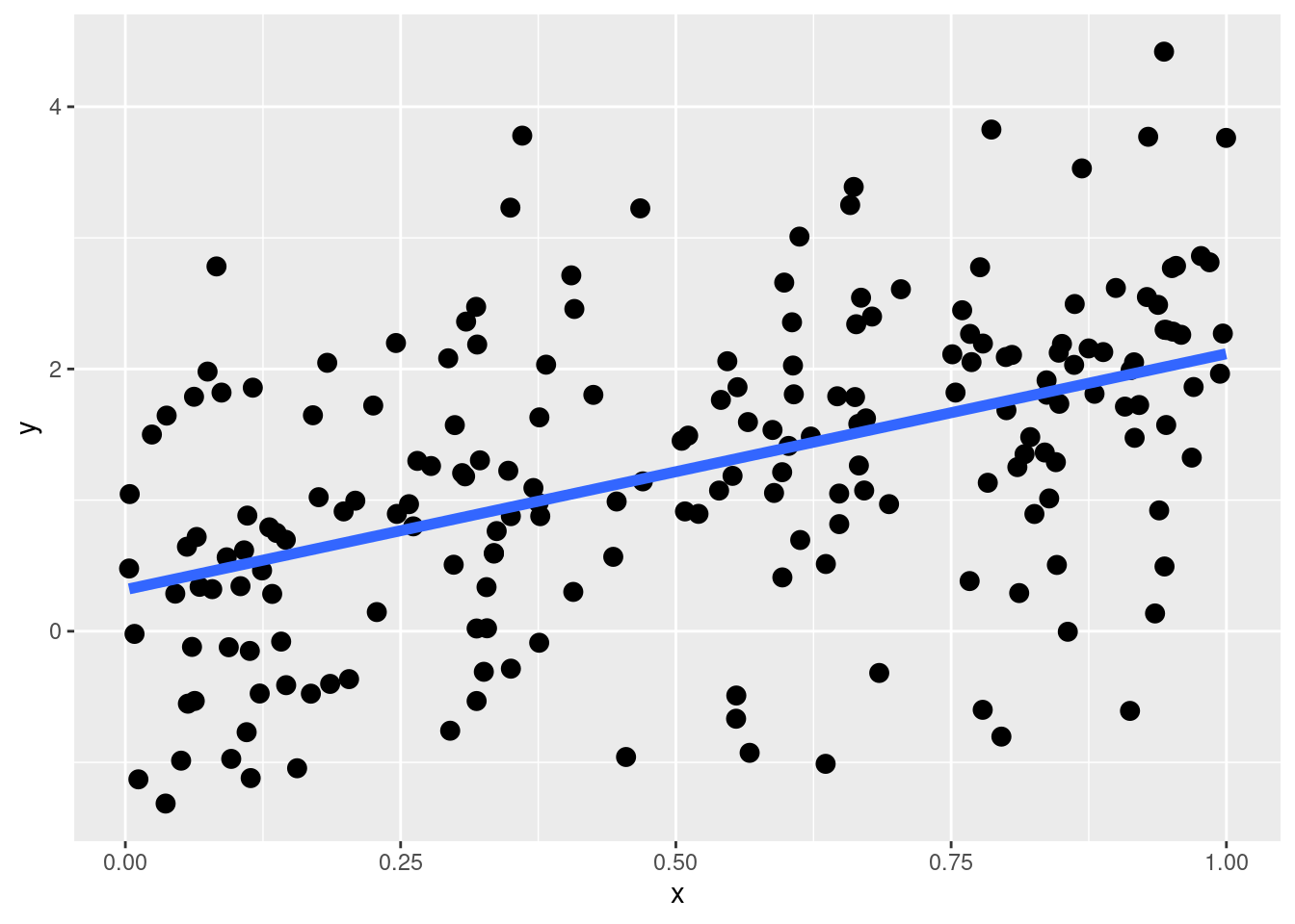
An important concept when learning Linear Models and Generalized Linear Models is understanding linear and non-linear effects. Starting from a linear effect let’s visualize a simple linear regression. \(x\) is a numerical predictor and the error term is Gaussian.
\[ y_i = \beta_0 + \beta_1x_i + \epsilon_i \]
Let’s simulate some data:
N <- 200
b0 <- 0.2
b1 <- 2
s <- 1
x <- runif(N, 0, 1)
y <- rnorm(N, b0 + b1 * x, s)
data.frame(x, y) |>
ggplot(aes(x = x, y = y)) +
geom_point(size = 3) +
geom_smooth(method = "lm", se = FALSE, formula = y ~ x, lwd = 2)
This is a linear effect and by default, when we include a predictor in a linear model lm(y ~ ...) we are assuming that the effect is linear. What is the meaning of a linear effect? The actual meaning is that, regardless the level of \(x\), the expected increase in \(y\) is the same. In mathematical terms, this means that the derivative \(\frac{dy}{dx}\) is constant for all \(x\) levels.
\[ \frac{dy}{dx} = \beta_1 \qquad \text{for all } x \]
\[ y = \beta_0 + \beta_1 x \quad \Longrightarrow \quad \frac{d}{dx}(\beta_0 + \beta_1 x) = \beta_1. \]
We can see this by plotting predictions and calculating the difference in \(y\):
dat <- data.frame(x, y)
fit <- lm(y ~ x, data = dat)
fit
Call:
lm(formula = y ~ x, data = dat)

Coefficients:
(Intercept)            x
      0.317        1.799
# two dataframes of two rows. same increase in x 0.05 in two different positions along the x line
nx <- list(
data.frame(x = c(0.25, 0.30)),
data.frame(x = c(0.60, 0.65))
)
pp <- lapply(nx, function(x) predict(fit, newdata = x))
pp[[1]]
1 2
0.7668470 0.8568113
[[2]]
1 2
1.396597 1.486561 # then we calculate the differences i.e. the derivative
sapply(pp, diff) 2 2
0.0899643 0.0899643 The differences are the same for the same increase in \(x\): this is a linear effect.
In GLMs, the effects are by default linear only in the link function scale. For example, in a Poisson model the effect of \(x\) (similarly to the previous example) is not usually linear due to the bounds of the Poisson distribution. In fact, using a log link function the effects are linear on the log scale but multiplicative on the Poisson scale.
Let’s simulate other data for a Poisson model:
lp <- log(5) + log(7) * x
y <- rpois(N, exp(lp))

data.frame(
    x, lp, y
)  |> ggplot(aes(x = x, y = y)) +
    geom_point() +
    geom_smooth(method = "glm", formula = y ~ x, se = FALSE, method.args = list(family = poisson))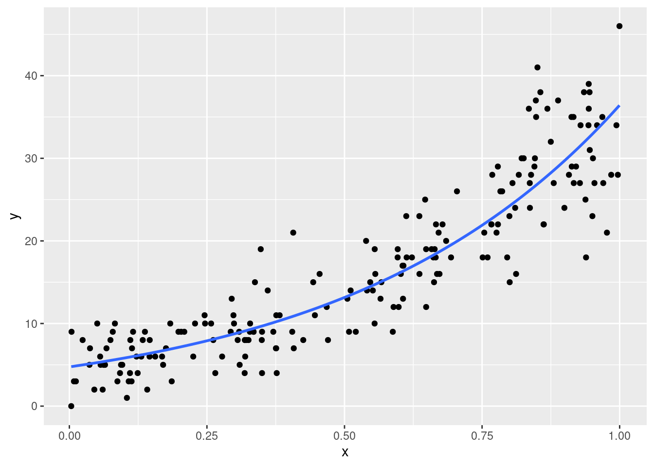
Clearly the effect is not linear. This means that for a given increase in \(x\), the increase in \(y\) is not constant. This increases the complexity in parameters interpretations. For example:
dat <- data.frame(x, y)
fit <- glm(y ~ x, data = dat, family = poisson(link = "log"))
fit
Call:  glm(formula = y ~ x, family = poisson(link = "log"), data = dat)

Coefficients:
(Intercept)            x
      1.558        2.037

Degrees of Freedom: 199 Total (i.e. Null);  198 Residual
Null Deviance:      1323
Residual Deviance: 223  AIC: 1105
# this is the increase in log(lambda) for a unit increase in x
# if x increases in 1 point, log(lambda) increases of b1
coef(fit)[2] x
2.037178 # this is the multiplicative increase in lambda for a unit increase in x
# if x increases in 1 point, lambda increases of 6.87 times
exp(coef(fit)[2]) x
7.66894 pp_log <- predict(fit, newdata = data.frame(x = c(0, 1)), type = "link")
diff(pp_log) # same as b1 2
2.037178 pp <- predict(fit, newdata = data.frame(x = c(0, 1)), type = "response")
pp[2] / pp[1] # same as exp(b1) 2
7.66894 Clearly, if we move to other \(x\) values, only the expected difference in \(\lambda\) changes while the difference on the log scale is constant because the GLM on the link function scale is linear.
# log scale, linear effect
diff(predict(fit, newdata = data.frame(x = c(0, 0.5))))
2
1.018589 diff(predict(fit, newdata = data.frame(x = c(0.5, 1)))) 2
1.018589 # lambda scale, non linear effect
diff(predict(fit, newdata = data.frame(x = c(0, 0.5)), type = "response")) 2
8.404801 diff(predict(fit, newdata = data.frame(x = c(0.5, 1)), type = "response")) 2
23.27529