Binomial GLM

Psychological Sciences

Filippo Gambarota

University of Padova

Last modified: 08-12-2025

Example: Passing the exam

We want to measure the impact of watching tv-shows on the probability of passing the statistics exam.

• exam: passing the exam (1 = “passed”, 0 = “failed”)
• tv_shows: watching tv-shows regularly (1 = “yes”, 0 = “no”)

id	tv_shows	h_study	coffee	presence	eta	mu	passed	age	faculty
1	1	27	4	1	-2.04	0.115	0	21	art
2	1	19	4	0	-3.28	0.036	0	23	ing
3	1	20	4	1	-2.6	0.069	0	21	med
4	1	20	7	1	-1.7	0.154	0	23	psy
...	...	...	...	...	...	...	...	...	...
97	0	69	2	0	1.72	0.848	1	24	art
98	0	69	0	1	3.02	0.953	1	19	med
99	0	66	0	1	2.78	0.942	1	22	med
100	0	53	2	1	1.94	0.874	1	23	art

Example: Passing the exam

We can create the contingency table

xtabs(~passed + tv_shows, data = exam) |> 
    addmargins()

#>       tv_shows
#> passed   0   1 Sum
#>    0     7  45  52
#>    1    43   5  48
#>    Sum  50  50 100

Example: Passing the exam

Each cell probability \(p_{ij}\) is computed as \(p_{ij}/n\)

(xtabs(~passed + tv_shows, data = exam)/nrow(exam)) |> 
    addmargins()

#>       tv_shows
#> passed    0    1  Sum
#>    0   0.07 0.45 0.52
#>    1   0.43 0.05 0.48
#>    Sum 0.50 0.50 1.00

Example: Passing the exam - Odds

The most common way to analyze a 2x2 contingency table is using the odds ratio (OR). Firsly let’s define the odds of success as:

\[ \begin{align*} odds = \frac{p}{1 - p} \\ p = \frac{odds}{odds + 1} \end{align*} \]

• the odds are non-negative, ranging between 0 and \(+\infty\)
• an odds of e.g. 3 means that we expect 3 success for each failure

Example: Passing the exam - Odds

For the exam example:

# odds <- function(p) p / (1 - p)
p11 <- mean(with(exam, passed[tv_shows == 1])) # passing exam | tv_shows
p11

#> [1] 0.1

odds(p11)

#> [1] 0.1111111

Example: Passing the exam - Odds Ratio

The OR is a ratio of odds:

\[ OR = \frac{\frac{p_1}{1 - p_1}}{\frac{p_2}{1 - p_2}} \]

• OR ranges between 0 and \(+\infty\). When \(OR = 1\) the odds for the two conditions are equal
• An e.g. \(OR = 3\) means that being in the condition at the numerator increase 3 times the odds of success

Example: Passing the exam - Odds Ratio

# or <- function(p1, p2) odds(p1) / odds(p2)
p11 <- mean(with(exam, passed[tv_shows == 1])) # passing exam | tv_shows
p10 <- mean(with(exam, passed[tv_shows == 0])) # passing exam | not tv_shows
p11

#> [1] 0.1

p10

#> [1] 0.86

or(p11, p10)

#> [1] 0.01808786

Why using these measure?

The odds have an interesting property when taking the logarithm. We can express a probability \(p\) using a scale ranging \([-\infty, +\infty]\)

Another example, Teddy Child

We considered a Study conducted by the University of Padua (TEDDY Child Study, 2020)¹. About post-partum depression. You can access the data using data("teddy") or within the data/ folder.

ID	Children	Fam_status	Education	Occupation	Age	Smoking_status	Alcool_status	Depression_pp	Parental_stress	Alabama_involvment	MSPSS_total	LTE	Partner_cohesion	Family_cohesion	Depression_pp01
1.000	1.000	Married	High school	Full-time	42.000	No	No	No	75.000	36.000	6.500	5.000	4.333	2.917	0.000
2.000	1.000	Married	High school	Full-time	42.000	No	No	No	51.000	41.000	5.500	5.000	4.167	3.000	0.000
3.000	1.000	Married	High school	Full-time	44.000	No	No	No	76.000	42.000	1.417	4.000	3.000	2.500	0.000
4.000	2.000	Married	High school	Full-time	48.000	No	No	No	88.000	39.000	1.083	4.000	2.167	2.667	0.000
5.000	3.000	Married	Degree or higher	Full-time	39.000	Yes	Yes	No	67.000	35.000	7.000	2.000	4.167	2.667	0.000
6.000	2.000	Married	Degree or higher	Full-time	38.000	Ex-smoker	No	No	61.000	36.000	3.333	0.000	3.000	2.583	0.000

1. Thanks to Prof. Paolo Girardi for the example, see https://teddychild.dpss.psy.unipd.it/ for information

Another example, Teddy Child

We want to see if the parental stress increase the probability of having post-partum depression:

Another example, Teddy Child

Another example, Teddy Child

Let’s start by fitting a linear model Depression_pp ~ Parental_stress. We consider “Yes” as 1 and “No” as 0.

fit_teddy_lm <- lm(Depression_pp01 ~ Parental_stress, data = teddy)
summary(fit_teddy_lm)

#> 
#> Call:
#> lm(formula = Depression_pp01 ~ Parental_stress, data = teddy)
#> 
#> Residuals:
#>      Min       1Q   Median       3Q      Max 
#> -0.42473 -0.13768 -0.10003 -0.05768  0.94702 
#> 
#> Coefficients:
#>                  Estimate Std. Error t value Pr(>|t|)    
#> (Intercept)     -0.172900   0.077561  -2.229 0.026389 *  
#> Parental_stress  0.004706   0.001201   3.919 0.000105 ***
#> ---
#> Signif. codes:  0 '***' 0.001 '**' 0.01 '*' 0.05 '.' 0.1 ' ' 1
#> 
#> Residual standard error: 0.3239 on 377 degrees of freedom
#> Multiple R-squared:  0.03915,    Adjusted R-squared:  0.0366 
#> F-statistic: 15.36 on 1 and 377 DF,  p-value: 0.0001054

Another example, Teddy Child

Let’s add the fitted line to our plot:

Another example, Teddy Child

… and check the residuals, pretty bad right?

Another example, Teddy Child

As for the exam example, we could compute a sort of contingency table despite the Parental_stress is a numerical variable by creating some discrete categories (just for exploratory analysis):

table(teddy$Depression_pp, teddy$Parental_stress_c) |> 
    round(2)

#>      
#>       < 40 40-60 60-80 80-100 > 100
#>   No     0   164   136     26     6
#>   Yes    0    15    21      7     4

table(teddy$Depression_pp, teddy$Parental_stress_c) |> 
    prop.table(margin = 2) |> 
    round(2)

#>      
#>       < 40 40-60 60-80 80-100 > 100
#>   No        0.92  0.87   0.79  0.60
#>   Yes       0.08  0.13   0.21  0.40

Another example, Teddy Child

Ideally, we could compute the increase in the odds of having the post-partum depression as the parental stress increase. In fact, as we are going to see, the Binomial GLM is able to estimate the non-linear increase in the probability.

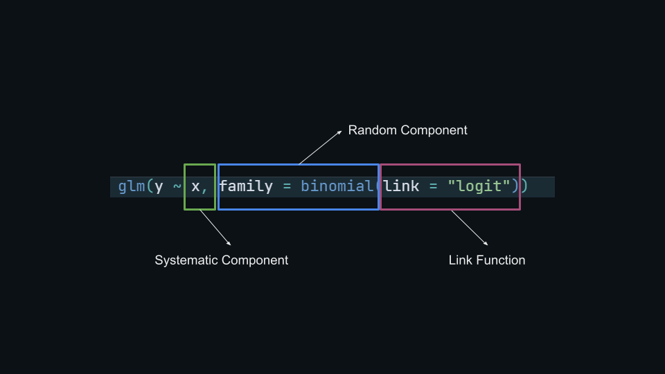
Binomial GLM

\[ \begin{aligned} y_i m_i &\sim \mathrm{Binomial}(\mu_i, m_i) \quad && \text{Random component} \\ \mbox{log} \frac{\mu_i}{1 - \mu_i} &= \beta_0 + \beta_1 x_{1i} + \dots + \beta_{p'} x_{p'i} \quad && \text{Systematic component} \end{aligned} \]

If you see the details about the Binomial distribution, \(\mu = pm\) where \(p\) is the probabiluty of success and \(m\) the number of trials. When \(m = 1\) we have the special case of a Bernoulli distribution. In this case we have \(n\) (\(n\) is the sample size) independent Bernoulli distributions.

Binomial GLM

• The random component of a Binomial GLM the binomial distribution with parameter \(p\)
• The systematic component is a linear combination of predictors and coefficients \(\boldsymbol{\beta X}\)
• The link function is a function that map probabilities into the \([-\infty, +\infty]\) range.

Logit Link

The logit link is the most common link function when using a binomial GLM:

\[ log \left(\frac{p_i}{1 - p_i}\right) = \beta_0 + \beta_1x_{i1} + \beta_2x_{i2} + \cdots + \beta_px_{ip} \]

The inverse of the logit maps again the probability into the \([0, 1]\) range:

\[ p = \frac{e^{\beta_0 + \beta_1x_{i1} + \beta_2x_{i2} + \cdots + \beta_px_{ip}}}{1 + e^{\beta_0 + \beta_1x_{i1} + \beta_2x_{i2} + \cdots + \beta_px_{ip}}} \]

Logit Link

Thus with a single numerical predictor \(x\) the relationship between \(x\) and \(p\) in non-linear on the probability scale but linear on the logit scale.

Logit Link

The main problem when using the logit link (and any link function beyond the identity) is that effects are linear on the link function scale but non-linear on the response scale.

Model fitting in R

The big picture…

Model fitting in R

We can model the contingency table presented before. We put data in binary form:

#>       tv_shows
#> passed  0  1
#>      0  7 45
#>      1 43  5

#> # A tibble: 9 × 10
#>   id    tv_shows h_study coffee presence eta   mu    passed age   faculty
#>   <chr> <chr>    <chr>   <chr>  <chr>    <chr> <chr> <chr>  <chr> <chr>  
#> 1 1     1        27      4      1        -2.04 0.115 0      21    art    
#> 2 2     1        19      4      0        -3.28 0.036 0      23    ing    
#> 3 3     1        20      4      1        -2.6  0.069 0      21    med    
#> 4 4     1        20      7      1        -1.7  0.154 0      23    psy    
#> 5 ...   ...      ...     ...    ...      ...   ...   ...    ...   ...    
#> 6 97    0        69      2      0        1.72  0.848 1      24    art    
#> 7 98    0        69      0      1        3.02  0.953 1      19    med    
#> 8 99    0        66      0      1        2.78  0.942 1      22    med    
#> 9 100   0        53      2      1        1.94  0.874 1      23    art

Intercept only model

Let’s start from the simplest model (often called null model) where there are no predictors:

fit0_exam <- glm(passed ~ 1, data = exam, family = binomial(link = "logit"))
summary(fit0_exam)

#> 
#> Call:
#> glm(formula = passed ~ 1, family = binomial(link = "logit"), 
#>     data = exam)
#> 
#> Coefficients:
#>             Estimate Std. Error z value Pr(>|z|)
#> (Intercept) -0.08004    0.20016    -0.4    0.689
#> 
#> (Dispersion parameter for binomial family taken to be 1)
#> 
#>     Null deviance: 138.47  on 99  degrees of freedom
#> Residual deviance: 138.47  on 99  degrees of freedom
#> AIC: 140.47
#> 
#> Number of Fisher Scoring iterations: 3

Intercept only model

When fitting an intercept-only model, the parameter is the average value of the y variable:

\[ \begin{align*} \log(\frac{p}{1 - p}) = \beta_0 \\ p = \frac{e^{\beta_0}}{1 + e^{\beta_0}} \end{align*} \]

Intercept only model

In R, the \(logit(p)\) is computed using qlogis() that is the q + logis combination of functions to work with probability distributions. The \(logit^{-1}\) thus the inverse of the logit function is plogis():

# average y on the respo nse scale
mean(exam$passed)

#> [1] 0.48

c("logit" = coef(fit0_exam)[1],
  "inv-logit" = plogis(coef(fit0_exam)[1])
)

#>     logit.(Intercept) inv-logit.(Intercept) 
#>           -0.08004271            0.48000000

Link function (TIPS)

If you are not sure about how to transform using the link function you can directly access the family() object in R that contains the appropriate link function and the corresponding inverse.

bin <- binomial(link = "logit")
bin$linkfun() # the same as qlogis
bin$linkinv() # the same as plogis

Model with \(X\)

Now we can add the tv_shows predictor. Now the model has two coefficients. Given that the tv_shows is a binary variable, the intercept is the average y when tv_shows is 0, and the tv_shows coefficient is the increase in y for a unit increase in tv_shows:

fit_exam <- glm(passed ~ tv_shows, data = exam, family = binomial(link = "logit"))
summary(fit_exam)

#> 
#> Call:
#> glm(formula = passed ~ tv_shows, family = binomial(link = "logit"), 
#>     data = exam)
#> 
#> Coefficients:
#>             Estimate Std. Error z value Pr(>|z|)    
#> (Intercept)   1.8153     0.4076   4.454 8.43e-06 ***
#> tv_shows1    -4.0125     0.6231  -6.439 1.20e-10 ***
#> ---
#> Signif. codes:  0 '***' 0.001 '**' 0.01 '*' 0.05 '.' 0.1 ' ' 1
#> 
#> (Dispersion parameter for binomial family taken to be 1)
#> 
#>     Null deviance: 138.469  on 99  degrees of freedom
#> Residual deviance:  73.005  on 98  degrees of freedom
#> AIC: 77.005
#> 
#> Number of Fisher Scoring iterations: 4

Model with \(X\)

Thinking about our data, the (Intercept) is the probability of passing the exam without watching tv-shows. The tv_shows (should be) the difference in the probability of passing the exam between people who watched or did not watched tv-shows, BUT:

• we are on the logit scale. Thus we are modelling log(odds) and not probabilities
• a difference on the log scale is a ratio on the raw scale. Thus taking the exponential of tv_shows we obtain the ratio of odds of passing the exam watching vs non-watching tv-shows. Do you remember something?

Model with \(X\)

The tv_shows is exactly the Odds Ratio that we calculated on the contingency table:

# from model coefficients
exp(coef(fit_exam)["tv_shows1"])

#>  tv_shows1 
#> 0.01808786

# from the contingency table
or(mean(exam$passed[exam$tv_shows == 1]),
   mean(exam$passed[exam$tv_shows == 0]))

#> [1] 0.01808786

Binomial vs Binary

There are several practical differences between binomial and binary models:

• data structure
• fitting function in R
• residuals and residual deviance
• type of predictors

Binomial vs Binary data structure

The most basic Binomial regression is a vector of binary \(y\) values and a continuous or categorical predictor. Let’s see a common data structure in this case:

n <- 30
df <- data.frame(id = 1:n)
df$x <- sim_n_x(df, list(level = "obs", f = runif))
b0 <- qlogis(0.01)
b1 <- 8

df |> 
    sim_data(~x, c(b0, b1), family = binomial(), which.mu = "prob", rng.arg = list(size = 1)) |> 
    select(id, x, y) |> 
    filor::trim_df(n = 4)

#> # A tibble: 9 × 3
#>   id    x     y    
#>   <chr> <chr> <chr>
#> 1 1     0.881 1    
#> 2 2     0.495 0    
#> 3 3     0.837 1    
#> 4 4     0.541 0    
#> 5 ...   ...   ...  
#> 6 27    0.981 1    
#> 7 28    0.001 0    
#> 8 29    0.488 0    
#> 9 30    0.455 0

Binomial vs Binary data structure

Or equivalently with a categorical variable:

n <- 15
x <- c("a", "b")
df <- sim_design(n, between = list(x = x))
b0 <- qlogis(0.4)
b1 <- log(or(0.7, 0.4))

df |> 
    sim_data(formula = ~x, beta = c(b0, b1), which.mu = "prob", family = binomial(), rng.arg = list(size = 1)) |> 
    dplyr::select(id, x, y) |> 
    filor::trim_df(4)

#> # A tibble: 9 × 3
#>   id    x     y    
#>   <chr> <chr> <chr>
#> 1 1     a     0    
#> 2 2     a     1    
#> 3 3     a     0    
#> 4 4     a     0    
#> 5 ...   ...   ...  
#> 6 27    b     1    
#> 7 28    b     1    
#> 8 29    b     1    
#> 9 30    b     1

Binomial vs Binary data structure

When using a Binomial data structure we count the number of success for each level of \(x\). nc is the number of 1 responses, nf is the number of 0 response out of nt trials:

x <- seq(0, 1, 0.05)
nt <- 10
nc <- rbinom(length(x), nt, plogis(qlogis(0.01) + 8*x))
dat <- data.frame(x, nc, nf = nt - nc,  nt)

dat |> 
    filor::trim_df(4)

#> # A tibble: 9 × 4
#>   x     nc    nf    nt   
#>   <chr> <chr> <chr> <chr>
#> 1 0     0     10    10   
#> 2 0.05  0     10    10   
#> 3 0.1   0     10    10   
#> 4 0.15  1     9     10   
#> 5 ...   ...   ...   ...  
#> 6 0.85  8     2     10   
#> 7 0.9   10    0     10   
#> 8 0.95  8     2     10   
#> 9 1     10    0     10

Binomial vs Binary data structure

With a categorical variable we have essentially a contingency table:

x <- c("a", "b")
nt <- 10
nc <- rbinom(length(x), nt, plogis(qlogis(0.4) + log(or(0.7, 0.4))*ifelse(x == "a", 1, 0)))

datc <- data.frame(x, nc, nf = nt - nc,  nt)
datc

#> # A tibble: 2 × 4
#>   x        nc    nf    nt
#>   <chr> <int> <dbl> <dbl>
#> 1 a         8     2    10
#> 2 b         5     5    10

Binomial vs Binary: data structure

Clearly, expanding or aggregating data is the way to convert a binary into a binomial data structure and the opposite:

# from binomial to binary
bin2binary(datc, nc, nt) |> 
    select(y, x) |> 
    filor::trim_df()

#> # A tibble: 9 × 2
#>   y     x    
#>   <chr> <chr>
#> 1 1     a    
#> 2 1     a    
#> 3 1     a    
#> 4 1     a    
#> 5 ...   ...  
#> 6 0     b    
#> 7 0     b    
#> 8 0     b    
#> 9 0     b

Binomial vs Binary: data structure

# from binary to binomial
bin2binary(datc, nc, nt)  |>
    binary2bin(y ~ x)

#> # A tibble: 2 × 4
#>   x        nc    nt    nf
#>   <chr> <dbl> <dbl> <dbl>
#> 1 a         8    10     2
#> 2 b         5    10     5

Binomial vs Binary: multilevel disclaimer

• Clearly, in the previous examples, each row correspond to a single observation (in the binary model) or a condition (in the binomial model). Furthermore each row/observation/participants is assumed to be independent.
• If participants performed multiple trials for each condition, we can still use a binomial or binary model BUT we need to take into account the multilevel structure.
• In practice, we need to use a mixed-effects GLM, for example with the lme4::glmer() package specifying the appropriate random structure.

Binomial vs Binary: - fitting function in R

There is a single way to implement a binary model in R and two ways for the binomial version:

# binary regression
glm(y ~ x, family = binomial(link = "logit"))

# binomial with cbind syntax, nc = number of 1s, nf = number of 0s, nc + nf = nt
glm(cbind(nc, nf) ~ x, family = binomial(link = "logit"))

# binomial with proportions and weights, equivalent to the cbind approach, nt is the total trials
glm(nc/nt ~ x, weights = nt, binomial(link = "logit"))

Binomial vs Binary: residuals and residual deviance

A more relevant difference is about the residual analysis. The binary regression has different residuals compared to the binomial model fitted on the same dataset¹.

fit_binomial <- glm(nc/nt ~ x, weights = nt, data = dat_binomial, family = binomial(link = "logit"))
fit_binary <- glm(y ~ x, data = dat_binary, family = binomial(link = "logit"))

1. To note, the binned residuals could be considered as an attempt to mitigate the binary residuals problem by creating bins of fitted/residual values similarly to fitting a binomial model.

Binomial vs Binary: residuals and residual deviance

Binomial vs Binary: residuals and residual deviance

The residual deviance is also different. In fact, there is more residual deviance on the binary compared to the binomial model. However, comparing two binary and binomial models actually leads to the same conclusion. In other terms the deviance seems to be on a different scale¹:

fit0_binary <- update(fit_binary, . ~ -x) # null binary model
fit0_binomial <- update(fit_binomial, . ~ -x) # null binary model

1. Thanks to Prof. Altoè for this suggestion

Binomial vs Binary: residuals and residual deviance

In fact, if we compare the full model with the null model in both binary and binomial version, the LRT is the same but the deviance is on a different scale. Comparing a binary with a binomial model could be completely misleading.

anova(fit_binomial, fit0_binomial, test = "Chisq")
#> # A tibble: 2 × 5
#>   `Resid. Df` `Resid. Dev`    Df Deviance `Pr(>Chi)`
#>         <dbl>        <dbl> <dbl>    <dbl>      <dbl>
#> 1          19         27.9    NA      NA   NA       
#> 2          20        158.     -1    -130.   3.24e-30
anova(fit_binary, fit0_binary, test = "Chisq")
#> # A tibble: 2 × 5
#>   `Resid. Df` `Resid. Dev`    Df Deviance `Pr(>Chi)`
#>         <dbl>        <dbl> <dbl>    <dbl>      <dbl>
#> 1         208         154.    NA      NA   NA       
#> 2         209         285.    -1    -130.   3.24e-30

Binomial vs Binary: type of predictors

This point is less relevant in this course but important in general. Usually, binary regression is used when the predictor is at the trial level whereas binomial regression is used when the predictor is at the participant level. When both levels are of interests one should use a mixed-effects model where both levels can be modeled.

• the probability of correct responses during an exam as a function of the question difficulty (each trial/row could have a different \(x\) level)
• the probability of passing the exam as a function of the high-school background regardless of having multiple trials, each trial/row has the same \(x_i\) for the participant \(i\)

Binomial vs Binary: type of predictors

The probability of correct responses during an exam as a function of the question difficulty

• each question (i.e., trial) has a 0/1 response and a difficulty level
• we are modelling a single participant, otherwise we need a multilevel (mixed-effects) model

Binomial vs Binary: type of predictors

dat <- expand_grid(id = 1, question = 1:30)
dat$y <- rbinom(nrow(dat), 1, 0.7)
dat$difficulty <- sample(1:5, nrow(dat), replace = TRUE)

dat |> 
    select(id, question, difficulty, y) |> 
    filor::trim_df()

#> # A tibble: 9 × 4
#>   id    question difficulty y    
#>   <chr> <chr>    <chr>      <chr>
#> 1 1     1        4          0    
#> 2 1     2        4          1    
#> 3 1     3        4          1    
#> 4 1     4        4          1    
#> 5 ...   ...      ...        ...  
#> 6 1     27       1          1    
#> 7 1     28       2          1    
#> 8 1     29       4          0    
#> 9 1     30       2          0

Binomial vs Binary: type of predictors

the probability of passing the exam as a function of the high-school background

• each “background” has different students that passed or not the exam (0/1)

Binomial vs Binary: type of predictors

#> # A tibble: 4 × 4
#>   background nc    nf    nt   
#>   <chr>      <chr> <chr> <chr>
#> 1 math       20    10    30   
#> 2 chemistry  13    7     20   
#> 3 art        10    0     10   
#> 4 sport      15    5     20

Or the binary version:

#> # A tibble: 9 × 5
#>   background nc    nf    nt    y    
#>   <chr>      <chr> <chr> <chr> <chr>
#> 1 math       20    10    30    1    
#> 2 math       20    10    30    1    
#> 3 math       20    10    30    1    
#> 4 math       20    10    30    1    
#> 5 ...        ...   ...   ...   ...  
#> 6 sport      15    5     20    0    
#> 7 sport      15    5     20    0    
#> 8 sport      15    5     20    0    
#> 9 sport      15    5     20    0

Binomial vs Binary: type of predictors

• To note that despite we can convert between the binary/binomial, the two models are not always the same. The high-school background example can be easily modelled either with a binary or binomial model because the predictor is at the participant level that coincides with the trial level.
• On the other side, the question difficulty example can only be modelled using a binary regression because each trial (0/1) has a different value for the predictor
• To include both predictors or to model multiple participants on the question difficulty example we need a mixed-effects model where both levels together with the repeated-measures can be handled.
• a very clear overview of this topic can be found here https://www.rensvandeschoot.com/tutorials/generalised-linear-models-with-glm-and-lme4/

Probit link

Probit link

• The mostly used link function when using a binomial GLM is the logit link. The probit link is another link function that can be used. The overall approach is the same between logit and probit models. The only difference is the parameter interpretation (i.e., no odds ratios) and the specific link function (and the inverse) to use.
• The probit model use the cumulative normal distribution but the actual difference with a logit functions is neglegible.

Probit link

Probit link

When using the probit link the parameters are interpreted as difference in z-scores associated with a unit increase in the predictors. In fact probabilities are mapped into z-scores using the cumulative normal distribution.

p1 <- 0.7
p2 <- 0.5

qlogis(c(p1, p2)) # log(odds(p1)), logit link

#> [1] 0.8472979 0.0000000

qnorm(c(p1, p2)) # probit link

#> [1] 0.5244005 0.0000000

log(or(p1, p2)) # ~ beta1, logit link

#> [1] 0.8472979

pnorm(p1) - pnorm(p2) # ~beta1, probit link

#> [1] 0.06657389

Probit link

Parameter Intepretation

Model Intepretation

Parameters and effects interpretation is probably the hardest part of GLMs. The main reason is the non linearity of response vs the linearity of the link function. We have few options:

• intepreting model coefficients directly or after transforming to known values (e.g., odds ratios)
• intepreting predictions on the response scale
• marginal effects

Intepreting model coefficients

Models coefficients are interpreted in the same way as standard regression models. The big difference concerns:

• numerical predictors
• categorical predictors

Using contrast coding and centering/standardizing we can make model coefficients easier to intepret.

Categorical predictors

We use a categorical predictor with \(k\) levels, the model will estimate \(k - 1\) parameters. The interpretation of these parameters depends on the contrast coding. In R the default is the treatment coding (or dummy coding). We can see the coding scheme using the model.matrix() function that return the \(\mathbf{X}\) matrix:

#>     (Intercept) tv_shows1
#> 1             1         1
#> 2             1         1
#> 3             1         1
#> 4             1         1
#> 5             1         1
#> 6             1         1
#> 95            1         0
#> 96            1         0
#> 97            1         0
#> 98            1         0
#> 99            1         0
#> 100           1         0

Categorical predictors

For the exam dataset, \(\beta_0\) is the reference level (default to 0 because is the first) and \(\beta_1\) is the difference between the second level and the reference level. Using, for example, the sum-to-zero coding we can change the \(\beta_0\) intepretation.

exam$tv_shows0 <- ifelse(exam$tv_shows == 0, -0.5, 0.5)
fit <- glm(passed ~ tv_shows0, data = exam, family = binomial(link = "logit"))

Categorical predictors

# grand mean
mean(c(mean(exam$passed[exam$tv_shows == 1]), mean(exam$passed[exam$tv_shows == 0])))

#> [1] 0.48

# intercept
plogis(coef(fit)[1])

#> (Intercept) 
#>   0.4524027

Categorical predictors

Numerical predictors

With numerical predictors the interpretation is less straightforward. Effects are linear only the logit scale. \(\beta_1\) is the increase in log-odds (of \(y\)) for a unit increase in \(x\) keeping fixed all other \(x\) s. Taking the inverse of the link function, \(e^{\beta_1}\) is the increase in odds ratio for a unit increase in \(x\).

Numerical predictors

Numerical predictors, centering and scaling

If we remove a constant value from a numerical predictor we are centering on that value. Usually we center on the mean, but other values are still possible. Centering affects only the intepretation of the constant terms, thus \(\beta_0\).

Standardizing requires dividing (and most of the time also centering) the predictor. Usually we standardize using the standard deviation of the predictor. This transform the predictor in standard deviation units.

\[ x_{i_0} = x_i - \bar x \]

\[ x_{i_z} = \frac{x_i - \bar x}{\sigma_x} \]

Numerical predictors

Numerical predictors

Let’s return to our teddy child example and fitting the proper model:

fit_glm <- glm(Depression_pp01 ~ Parental_stress, data = teddy, family = binomial(link = "logit"))
summary(fit_glm)

#> 
#> Call:
#> glm(formula = Depression_pp01 ~ Parental_stress, family = binomial(link = "logit"), 
#>     data = teddy)
#> 
#> Coefficients:
#>                  Estimate Std. Error z value Pr(>|z|)    
#> (Intercept)     -4.323906   0.690689  -6.260 3.84e-10 ***
#> Parental_stress  0.036015   0.009838   3.661 0.000251 ***
#> ---
#> Signif. codes:  0 '***' 0.001 '**' 0.01 '*' 0.05 '.' 0.1 ' ' 1
#> 
#> (Dispersion parameter for binomial family taken to be 1)
#> 
#>     Null deviance: 284.13  on 378  degrees of freedom
#> Residual deviance: 271.23  on 377  degrees of freedom
#> AIC: 275.23
#> 
#> Number of Fisher Scoring iterations: 5

Numerical predictors

The (Intercept) (\(\beta_0\)) is the probability of having post-partum depression for a mother with parental stress zero (maybe better centering?)

\[ p(yes|x = 0) = g^{-1}(\beta_0) \]

plogis(coef(fit_glm)["(Intercept)"])

#> (Intercept) 
#>  0.01307482

Numerical predictors

The Parental_stress (\(\beta_1\)) is the increase in the \(log(odds)\) of having the post-partum depression for a unit increase in the parental stress index. If we take the exponential of \(\beta_1\) we obtain the increase in the \(odds\) of having post-partum depression for a unit increase in parental stress index.

exp(coef(fit_glm)["Parental_stress"])

#> Parental_stress 
#>        1.036671

Numerical predictors

The problem is that, as shown before, the effects are non-linear on the probability scale while are linear on the logit scale. On the logit scale, all differences are constant:

pr <- list(c(10, 11), c(50, 51), c(70, 71))

predictions <- lapply(pr, function(x) {
    predict(fit_glm, newdata = data.frame(Parental_stress = x))
})

# notice that the difference is exactly the Parental_stress parameter
sapply(predictions, diff)

#>         2         2         2 
#> 0.0360147 0.0360147 0.0360147

Numerical predictors

While on the probability scale, the differences are not the same. This is problematic when interpreting the results of a Binomial GLM with a numerical predictor.

(predictions <- lapply(predictions, plogis))

#> [[1]]
#>          1          2 
#> 0.01863764 0.01930790 
#> 
#> [[2]]
#>          1          2 
#> 0.07424969 0.07676350 
#> 
#> [[3]]
#>         1         2 
#> 0.1415012 0.1459330

sapply(predictions, diff)

#>            2            2            2 
#> 0.0006702661 0.0025138036 0.0044317558

Predicted probabilities

In a similar way we can use the inverse logit function to find the predicted probability specific values of \(x\). For example, the difference between \(p(y = 1|x = 2.5) - p(y = 1|x = 5)\) can be calculated using the model equation:

• \(p(y = 1|x = 2.5) = \frac{e^{\beta_0 + \beta_1 2.5}}{1 + e^{\beta_0 + \beta_1 2.5}}\)
• \(p(y = 1|x = 5) = \frac{e^{\beta_0 + \beta_1 5}}{1 + e^{\beta_0 + \beta_1 5}}\)
• \(p(y = 1|x = 5) - p(y = 1|x = 2.5)\)

coefs <- coef(fit)
plogis(coefs[1] + coefs[2]*5) - plogis(coefs[1] + coefs[2]*2.5)

#>  (Intercept) 
#> 1.057591e-07

Predicted probabilities

In R we can use directly the predict() function with the argument type = "response" to return the predicted probabilities instead of the logits:

preds <- predict(fit, newdata = list(x = c(2.5, 5)), type = "response")
preds

#>         1         2 
#> 0.9999999 1.0000000

preds[2] - preds[1]

#>            2 
#> 1.057591e-07

Marginal effects: a really comprehensive framework

The marginaleffects package provide a very complete and comprehensive framework to compute marginal effects for several models. You can have a very detailed overview of the theory and the functions reading:

• The main paper by Arel-Bundock et al. (2024)
• https://www.youtube.com/watch?v=ANDC_kkAjeM

Marginal effects

The marginal effect is the change in the response variable for a tiny change in the predictor. Is the slope (or the derivative) for a given \(x\) value.

In standard linear models, effects are linear also in the response (identity link) thus we have a single slope/derivative by definition.

In GLMs we the rate of increase in \(y\) depends on the \(x\) value thus evaluating the effect on the response is more complicated.

The marginaleffects provides a very clear framework to evaluate these effects in several models including the GLMs.

Marginal effects

Let’s imagine a simple y ~ x relationship on the probability scale. For each different tiny increase in \(x\) we have an increase in \(y\).

Marginal effects

Now let’s plot all the red slopes and see what we can learn:

Marginal effects

The blue line is the average slope. In other terms is the average increase in \(y\) for an unit increase in \(x\). We can say that on average, an increase in \(x\) produces an increase of 0.1 in terms of probability.

The red dot is the maximal slope. In other terms is the maximal increase in \(y\) for a specific unit increse in \(x\). We can say that the maximal increase in \(y\) (~ 0.2) happens when \(x\) is ~ 5.7.

Marginal effects

These two ways of summarising a non-linear relationships are called respectively average marginal effect and maximal marginal effect.

For more complex models and multiple predictors there is the marginaleffects package.

Let’s use the teddychild dataset:

head(teddy)

#> # A tibble: 6 × 17
#>      ID Children Fam_status Education        Occupation   Age Smoking_status
#>   <int>    <int> <chr>      <chr>            <chr>      <int> <chr>         
#> 1     1        1 Married    High school      Full-time     42 No            
#> 2     2        1 Married    High school      Full-time     42 No            
#> 3     3        1 Married    High school      Full-time     44 No            
#> 4     4        2 Married    High school      Full-time     48 No            
#> 5     5        3 Married    Degree or higher Full-time     39 Yes           
#> 6     6        2 Married    Degree or higher Full-time     38 Ex-smoker     
#> # ℹ 10 more variables: Alcool_status <chr>, Depression_pp <chr>,
#> #   Parental_stress <int>, Alabama_involvment <int>, MSPSS_total <dbl>,
#> #   LTE <int>, Partner_cohesion <dbl>, Family_cohesion <dbl>,
#> #   Depression_pp01 <dbl>, Parental_stress_c <fct>

Marginal effects

fit_teddy <- glm(Depression_pp01 ~ Parental_stress, data = teddy, family = binomial(link = "logit"))
summary(fit_teddy)

#> 
#> Call:
#> glm(formula = Depression_pp01 ~ Parental_stress, family = binomial(link = "logit"), 
#>     data = teddy)
#> 
#> Coefficients:
#>                  Estimate Std. Error z value Pr(>|z|)    
#> (Intercept)     -4.323906   0.690689  -6.260 3.84e-10 ***
#> Parental_stress  0.036015   0.009838   3.661 0.000251 ***
#> ---
#> Signif. codes:  0 '***' 0.001 '**' 0.01 '*' 0.05 '.' 0.1 ' ' 1
#> 
#> (Dispersion parameter for binomial family taken to be 1)
#> 
#>     Null deviance: 284.13  on 378  degrees of freedom
#> Residual deviance: 271.23  on 377  degrees of freedom
#> AIC: 275.23
#> 
#> Number of Fisher Scoring iterations: 5

Marginal effects

plot(ggeffect(fit_teddy))

Marginal effects

We can use the slopes() function from the marginaleffects package. Basically we are calculating the slope for each \(x\) value in the dataset.

library(marginaleffects)
sl <- slopes(fit_teddy)
sl

#> 
#>  Estimate Std. Error    z Pr(>|z|)    S   2.5 %  97.5 %
#>   0.00496   0.001659 2.99  0.00281  8.5 0.00171 0.00821
#>   0.00255   0.000476 5.36  < 0.001 23.5 0.00162 0.00349
#>   0.00508   0.001725 2.94  0.00325  8.3 0.00170 0.00846
#>   0.00656   0.002514 2.61  0.00904  6.8 0.00164 0.01149
#>   0.00404   0.001168 3.46  < 0.001 10.9 0.00175 0.00633
#> --- 369 rows omitted. See ?print.marginaleffects ---
#>   0.00255   0.000476 5.36  < 0.001 23.5 0.00162 0.00349
#>   0.00404   0.001168 3.46  < 0.001 10.9 0.00175 0.00633
#>   0.00449   0.001404 3.20  0.00139  9.5 0.00174 0.00724
#>   0.00363   0.000954 3.80  < 0.001 12.7 0.00175 0.00550
#>   0.00438   0.001343 3.26  0.00113  9.8 0.00174 0.00701
#> Term: Parental_stress
#> Type: response
#> Comparison: dY/dX

Marginal effects

This is the same plot we did before but with the teddy dataset:

Marginal effects

We can calculate the same quantities directly with the marginaleffects package:

avg_slopes(fit_teddy)

#> 
#>  Estimate Std. Error   z Pr(>|z|)    S   2.5 %  97.5 %
#>   0.00375    0.00101 3.7   <0.001 12.2 0.00176 0.00574
#> 
#> Term: Parental_stress
#> Type: response
#> Comparison: dY/dX

filter(sl, estimate == max(estimate))

#> 
#>  Estimate Std. Error    z Pr(>|z|)    S  2.5 % 97.5 %
#>   0.00899    0.00229 3.92   <0.001 13.5 0.0045 0.0135
#> 
#> Term: Parental_stress
#> Type: response
#> Comparison: dY/dX

Marginal effects

With more predictors we can calculate marginal effects, controlling for other variables:

data(teddy)
teddy$Depression_pp01 <- ifelse(teddy$Depression_pp == "Yes", 1, 0)
fit_teddy <- glm(Depression_pp01 ~ Parental_stress + Family_cohesion, data = teddy, family = binomial(link = "logit"))
summary(fit_teddy)

#> 
#> Call:
#> glm(formula = Depression_pp01 ~ Parental_stress + Family_cohesion, 
#>     family = binomial(link = "logit"), data = teddy)
#> 
#> Coefficients:
#>                  Estimate Std. Error z value Pr(>|z|)    
#> (Intercept)     -7.898099   2.046838  -3.859 0.000114 ***
#> Parental_stress  0.036140   0.009921   3.643 0.000270 ***
#> Family_cohesion  1.249750   0.662557   1.886 0.059261 .  
#> ---
#> Signif. codes:  0 '***' 0.001 '**' 0.01 '*' 0.05 '.' 0.1 ' ' 1
#> 
#> (Dispersion parameter for binomial family taken to be 1)
#> 
#>     Null deviance: 284.13  on 378  degrees of freedom
#> Residual deviance: 267.60  on 376  degrees of freedom
#> AIC: 273.6
#> 
#> Number of Fisher Scoring iterations: 5

Marginal effects

Marginal effects

slopes(fit_teddy)

#> 
#>             Term Estimate Std. Error    z Pr(>|z|)    S    2.5 %  97.5 %
#>  Family_cohesion  0.18139   0.101423 1.79  0.07371  3.8 -0.01740 0.38017
#>  Family_cohesion  0.10302   0.064103 1.61  0.10802  3.2 -0.02262 0.22866
#>  Family_cohesion  0.12853   0.047042 2.73  0.00629  7.3  0.03633 0.22073
#>  Family_cohesion  0.20010   0.094914 2.11  0.03501  4.8  0.01407 0.38613
#>  Family_cohesion  0.11734   0.051358 2.28  0.02233  5.5  0.01668 0.21799
#> --- 748 rows omitted. See ?print.marginaleffects ---
#>  Parental_stress  0.00229   0.000461 4.97  < 0.001 20.5  0.00139 0.00319
#>  Parental_stress  0.00339   0.001060 3.20  0.00137  9.5  0.00132 0.00547
#>  Parental_stress  0.00350   0.001239 2.83  0.00469  7.7  0.00107 0.00593
#>  Parental_stress  0.00302   0.000872 3.46  < 0.001 10.9  0.00131 0.00473
#>  Parental_stress  0.00431   0.001342 3.22  0.00130  9.6  0.00168 0.00694
#> Type: response
#> Comparison: dY/dX

Marginal effects

avg_slopes(fit_teddy)

#> 
#>             Term Estimate Std. Error    z Pr(>|z|)    S    2.5 %  97.5 %
#>  Family_cohesion  0.12845     0.0681 1.89   0.0592  4.1 -0.00499 0.26188
#>  Parental_stress  0.00371     0.0010 3.70   <0.001 12.2  0.00175 0.00568
#> 
#> Type: response
#> Comparison: dY/dX

# Marginal Effect at the Mean (MEM)
slopes(fit_teddy, newdata = datagrid())

#> 
#>             Term Estimate Std. Error    z Pr(>|z|)    S    2.5 %  97.5 %
#>  Family_cohesion  0.12285   0.063917 1.92   0.0546  4.2 -0.00243 0.24812
#>  Parental_stress  0.00355   0.000949 3.74   <0.001 12.4  0.00169 0.00541
#> 
#> Type: response
#> Comparison: dY/dX

slopes(fit_teddy) |> 
    group_by(term) |> 
    summarise(estimate = max(estimate))

#> # A tibble: 2 × 2
#>   term            estimate
#>   <chr>              <dbl>
#> 1 Family_cohesion  0.311  
#> 2 Parental_stress  0.00899

Marginal means with emmeans

When using categorical variables, the emmeans package is more effective (despite the marginaleffects package can be used). The idea is to calculate the predicted probabilities for combinations of (categorical) predictors and eventually compute contrasts between means.

fit_teddy <- glm(Depression_pp01 ~ Education, data = teddy, family = binomial(link = "logit"))
summary(fit_teddy)

#> 
#> Call:
#> glm(formula = Depression_pp01 ~ Education, family = binomial(link = "logit"), 
#>     data = teddy)
#> 
#> Coefficients:
#>                        Estimate Std. Error z value Pr(>|z|)    
#> (Intercept)             -1.9315     0.2393  -8.073 6.87e-16 ***
#> EducationHigh school     0.0205     0.3212   0.064    0.949    
#> EducationMiddle school  -0.5942     0.7728  -0.769    0.442    
#> ---
#> Signif. codes:  0 '***' 0.001 '**' 0.01 '*' 0.05 '.' 0.1 ' ' 1
#> 
#> (Dispersion parameter for binomial family taken to be 1)
#> 
#>     Null deviance: 284.13  on 378  degrees of freedom
#> Residual deviance: 283.37  on 376  degrees of freedom
#> AIC: 289.37
#> 
#> Number of Fisher Scoring iterations: 5

Marginal means with emmeans

library(emmeans)
emmeans(fit_teddy, ~ Education)

#>  Education        emmean    SE  df asymp.LCL asymp.UCL
#>  Degree or higher  -1.93 0.239 Inf     -2.40     -1.46
#>  High school       -1.91 0.214 Inf     -2.33     -1.49
#>  Middle school     -2.53 0.735 Inf     -3.97     -1.09
#> 
#> Results are given on the logit (not the response) scale. 
#> Confidence level used: 0.95

emmeans(fit_teddy, ~ Education, type = "response")

#>  Education          prob     SE  df asymp.LCL asymp.UCL
#>  Degree or higher 0.1266 0.0265 Inf    0.0831     0.188
#>  High school      0.1289 0.0241 Inf    0.0886     0.184
#>  Middle school    0.0741 0.0504 Inf    0.0186     0.252
#> 
#> Confidence level used: 0.95 
#> Intervals are back-transformed from the logit scale

Inverse estimation¹

Sometimes it is useful to do what is called inverse estimation, thus predicting the \(x\) level associated with a certain \(y\). In this case the \(x\) producing a certain \(p\) of response.

Sometimes this is called median effective dose when finding the \(x\) level producing \(50\%\) of correct responses.

We can use the MASS::dose.p() function. Clearly, the range of the predictor need to be meaningful. Predicting the probability of post partum depression being 0.9 is probably meaningless given the bounded nature of the predictor variable.

1. see also the investr package

Inverse estimation

Still using the TeddyChild dataset, an application could be to estimate the level of parental stress required to have a certain probability of post-partum depression. For example:

fit_teddy <- glm(Depression_pp01 ~ Parental_stress, data = teddy, family = binomial(link = "logit"))
MASS::dose.p(fit_teddy, p = c(0.5, 0.7, 0.8))

#>              Dose       SE
#> p = 0.5: 120.0595 14.80923
#> p = 0.7: 143.5859 21.03040
#> p = 0.8: 158.5519 25.04193

Inverse estimation and Psychophysics

In Psychophysics it is common to do the inverse estimation to estimate the detection or performance threshold. For example, estimating the \(x\) level associated with a certain probability of success e.g. 50%.

curve(plogis(x, 0.7, 1/8), 
      ylim = c(0, 1),
      xlab = "Stimulus Contrast",
      ylab = "Probability of Detection",
      lwd = 2)
segments(x0 = 0.7, y0 = 0, x1 = 0.7, 0.5, lty = 2)
segments(x0 = 0, y0 = 0.5, x1 = 0.7, 0.5, lty = 2)
points(x = 0.7, y = 0.5, pch = 19, col = "firebrick", cex = 2)

Inverse estimation and Psychophysics

Let’s simulate and ideal observer that respond to stimuli with different contrast:

th <- 0.7 # -(b0/b1)
slope <- 1/8

b1 <- 1/slope
b0 <- -th*b1

x <- rep(seq(0, 1, 0.1), each = 20)

p <- plogis(b0 + b1 * x)
y <- rbinom(length(x), 1, p)

yp <- tapply(y, x, mean)
xc <- unique(x)

plot(xc, yp, type = "b", ylim = c(0, 1), xlab = "Contrast", ylab = "Probability of Detection")
curve(plogis(x, th, slope), add = TRUE, col = "firebrick", lwd = 2)

Inverse estimation and Psychophysics

fit <- glm(y ~ x, family = binomial(link = "logit"))
summary(fit)

#> 
#> Call:
#> glm(formula = y ~ x, family = binomial(link = "logit"))
#> 
#> Coefficients:
#>             Estimate Std. Error z value Pr(>|z|)    
#> (Intercept)  -5.0421     0.6762  -7.456 8.92e-14 ***
#> x             6.8045     0.9394   7.243 4.38e-13 ***
#> ---
#> Signif. codes:  0 '***' 0.001 '**' 0.01 '*' 0.05 '.' 0.1 ' ' 1
#> 
#> (Dispersion parameter for binomial family taken to be 1)
#> 
#>     Null deviance: 267.06  on 219  degrees of freedom
#> Residual deviance: 163.48  on 218  degrees of freedom
#> AIC: 167.48
#> 
#> Number of Fisher Scoring iterations: 6

Inverse estimation and Psychophysics

We can estimate the threshold and slope of the psychometric function using the equations from Knoblauch & Maloney (2012).

-(coef(fit)[1]/coef(fit)[2]) # threshold

#> (Intercept) 
#>   0.7410012

MASS::dose.p(fit, p = 0.5) # with inverse estimation

#>               Dose         SE
#> p = 0.5: 0.7410012 0.02964516

Odds Ratio (OR) to Cohen’s \(d\)

The Odds Ratio can be considered an effect size measure. We can transform the OR into other effect size measure (Borenstein et al., 2009; Sánchez-Meca et al., 2003).

\[ d = \log(OR) \frac{\sqrt{3}}{\pi} \]

# in R with the effectsize package
or <- 1.5
effectsize::logoddsratio_to_d(log(or))

#> [1] 0.2235446

# or 
effectsize::oddsratio_to_d(or)

#> [1] 0.2235446

Odds Ratio (OR) to Cohen’s \(d\)

References

Arel-Bundock, V., Greifer, N., & Heiss, A. (2024). How to Interpret Statistical Models Using marginaleffects for R and Python. Journal of Statistical Software, 111, 1–32. https://doi.org/10.18637/jss.v111.i09

Borenstein, M., Hedges, L. V., Higgins, J. P. T., & Rothstein, H. R. (2009). Introduction to Meta-Analysis. https://doi.org/10.1002/9780470743386

Knoblauch, K., & Maloney, L. T. (2012). Modeling Psychophysical Data in R. Springer New York. https://doi.org/10.1007/978-1-4614-4475-6

Sánchez-Meca, J., Marín-Martínez, F., & Chacón-Moscoso, S. (2003). Effect-size indices for dichotomized outcomes in meta-analysis. Psychological Methods, 8, 448–467. https://doi.org/10.1037/1082-989X.8.4.448