Gamma GLM

Psychological Sciences

Filippo Gambarota

University of Padova

Last modified: 26-01-2025

Gamma Distribution

Gamma distribution

The Gamma distribution has several :parametrizations. One of the most common is the shape-scale parametrization:

\[ f(x;k,\theta )={\frac {x^{k-1}e^{-x/\theta }}{\theta ^{k}\Gamma (k)}} \] Where \(\theta\) is the scale parameter and \(k\) is the shape parameter.

Gamma distribution

ggamma(mean = c(10, 20, 30), sd = c(10, 10, 10), show = "ss")

Gamma \(\mu\) and \(\sigma^2\)

The mean and variance are defined as:

• \(\mu = k \theta\) and \(\sigma^2 = k \theta^2\) with the shape-scale parametrization
• \(\mu = \frac{\alpha}{\beta}\) and \(\frac{\alpha}{\beta^2}\) with the shape-rate parametrization

Another important quantity is the coefficient of variation defined as \(\frac{\sigma}{\mu}\) or \(\frac{1}{\sqrt{k}}\) (or \(\frac{1}{\sqrt{\alpha}}\)).

Gamma distribution

Again, we can see the mean-variance relationship:

ggamma(shape = c(5, 5), scale = c(10, 20), show = "ss")

Gamma parametrization

To convert between different parametrizations, you can use the gamma_params() function:

gamma_params <- function(shape = NULL, scale = 1/rate, rate = 1,
                         mean = NULL, sd = NULL,
                         eqs = FALSE){
  if(eqs){
    cat(rep("=", 25), "\n")
    cat(eqs()$gamma, "\n")
    cat(rep("=", 25), "\n")
  }else{
      if(is.null(shape)){
      var <- sd^2
      shape <- mean^2 / var
      scale <- mean / shape
      rate <- 1/scale
    } else if(is.null(mean) & is.null(sd)){
      if(is.null(rate)){
        scale <- 1/rate
      } else{
        rate <- 1/scale
      }
      mean <- shape * scale
      var <- shape * scale^2
      sd <- sqrt(var)
    }else{
      stop("when shape and scale are provided, mean and sd need to be NULL (and viceversa)")
    }
    out <- list(shape = shape, scale = scale, rate = rate, mean = mean, var = var, sd = sd)
    # coefficient of variation
    out$cv <- 1/sqrt(shape)
    return(out)
  }
}

Gamma parametrization

gm <- gamma_params(mean = 30, sd = 10)
unlist(gm)

#>       shape       scale        rate        mean         var          sd 
#>   9.0000000   3.3333333   0.3000000  30.0000000 100.0000000  10.0000000 
#>          cv 
#>   0.3333333

y <- rgamma(1000, shape = gm$shape, scale = gm$scale)

Gamma parametrization

Understanding parameters

\(\mu\) and \(\sigma\) parametrization

• Using the gamma_params() function we can think in terms of \(\mu\) and \(\sigma\) and generate the right parameters (e.g., shape and rate).
• Let’s simulate observations from a Gamma distribution with \(\mu = 500\) and \(\sigma = 200\)

\(\mu\) and \(\sigma\) parametrization

Then we can fit an intercept-only model with the Gamma family and a log link function. You have to specify the link because the default is inverse.

fam <- Gamma(link = "log")
dat <- data.frame(y)
fit0 <- glm(y ~ 1, family = fam, data = dat)
summary(fit0)

#> 
#> Call:
#> glm(formula = y ~ 1, family = fam, data = dat)
#> 
#> Coefficients:
#>             Estimate Std. Error t value Pr(>|t|)    
#> (Intercept) 6.205013   0.003959    1567   <2e-16 ***
#> ---
#> Signif. codes:  0 '***' 0.001 '**' 0.01 '*' 0.05 '.' 0.1 ' ' 1
#> 
#> (Dispersion parameter for Gamma family taken to be 0.1567542)
#> 
#>     Null deviance: 1625.2  on 9999  degrees of freedom
#> Residual deviance: 1625.2  on 9999  degrees of freedom
#> AIC: 132959
#> 
#> Number of Fisher Scoring iterations: 4

\(\mu\) and \(\sigma\) parametrization

\(\beta_0\) is the \(\mu\) of the Gamma distribution. We need to apply the inverse (exp) to get the original scale:

c(mean = mean(dat$y), mean_true = gm$mean, b0 = exp(coef(fit0)[1]))

#>           mean      mean_true b0.(Intercept) 
#>       495.2254       500.0000       495.2254

as always you can use the fam() object if you are not sure about the link functions as fam$linkinv(coef(fit0)[1])

\(\mu\) and \(\sigma\) parametrization

Now let’s simulate the difference between two groups. Again fixing the \(\mu_0 = 500\), \(\mu_1 = 600\) and a common \(\sigma = 200\). Let’s plot the empirical densities:

ggamma(mean = c(500, 600), sd = c(200, 200))

\(\mu\) and \(\sigma\) parametrization

Using the group variable as dummy-coded, \(\beta_0 = \mu_0\) and \(\beta_1 = \mu_1 - \mu_0\). Note that we are in the log scale.

ns <- 1e4
m0 <- 500
m1 <- 600
s <- 200
# parameters, log link
b0 <- log(m0)
b1 <- log(m1) - log(m0) # equivalent to log(m1 / m0)
x <- rep(c(0, 1), each = ns/2)
lp <- b0 + b1 * x # linear predictor
mu <- exp(lp) # inverse exp link
gm <- gamma_params(mean = mu, sd = s)
y <- rgamma(ns, shape = gm$shape, scale = gm$scale)
dat <- data.frame(y, x)

\(\mu\) and \(\sigma\) parametrization

Let’s see the simulated data:

par(mfrow = c(1,2))
hist(dat$y, col = "dodgerblue", breaks = 100)
boxplot(y ~ x, data = dat)

\(\mu\) and \(\sigma\) parametrization

Now we can fit the model and extract the parameters:

fit <- glm(y ~ x, data = dat, family = fam)
summary(fit)

#> 
#> Call:
#> glm(formula = y ~ x, family = fam, data = dat)
#> 
#> Coefficients:
#>             Estimate Std. Error t value Pr(>|t|)    
#> (Intercept) 6.214269   0.005242 1185.58   <2e-16 ***
#> x           0.181938   0.007413   24.54   <2e-16 ***
#> ---
#> Signif. codes:  0 '***' 0.001 '**' 0.01 '*' 0.05 '.' 0.1 ' ' 1
#> 
#> (Dispersion parameter for Gamma family taken to be 0.1373681)
#> 
#>     Null deviance: 1486.5  on 9999  degrees of freedom
#> Residual deviance: 1403.8  on 9998  degrees of freedom
#> AIC: 133686
#> 
#> Number of Fisher Scoring iterations: 4

\(\mu\) and \(\sigma\) parametrization

\(\beta_0\) is the mean of the first group and \(\beta_1\) is the \(\log(\mu_1/\mu_0)\) or the difference \(\log(\mu_1) - log(\mu_0)\)

mm <- tapply(dat$y, dat$x, mean)
coefs <- coef(fit)
# manually
c(mm["0"], mm["1"], diff = log(mm["1"]) - log(mm["0"]))

#>           0           1      diff.1 
#> 499.8307000 599.5669342   0.1819382

# model
c(exp(coefs[1]), exp(coefs[1] + coefs[2]), coefs[2])

#> (Intercept) (Intercept)           x 
#> 499.8307000 599.5669342   0.1819382

\(\mu\) and \(\sigma\) parametrization

The other estimated parameter is the dispersion that is defined as the inverse of the shape. We have not a single shape but the average is roughly similar to the true value.

fits <- summary(fit)
fits$dispersion

#> [1] 0.1373681

1/mean(unique(gm$shape))

#> [1] 0.1311475

\(\mu\) and shape parametrization

This is common in brms and other packages¹. The \(\mu\) is the same as before and the shape (\(\alpha\)) determine the skewness of the distribution. For the Gamma, the skewness is calculated as \(\frac{2}{\sqrt{\alpha}}\).

To generate data, we calculate the scale (\(\theta\)) as \(\frac{\mu}{\alpha}\) (remember that \(\mu = \alpha\theta\))

mu <- 50
shape <- 10
y <- rgamma(1e4, shape = shape, scale = mu/shape)
hist(y, col = "dodgerblue", breaks = 100)

1. See an example https://rpubs.com/jwesner/gamma_glm

\(\mu\) and shape parametrization

the expected skewness is 2/sqrt(shape) 0.632 and is similar to the value computed on the simulated data

2/sqrt(shape)

#> [1] 0.6324555

psych::skew(y)

#> [1] 0.6141622

as \(\alpha\) increase, the Gamma distribution is less skewed and approaches a Gaussian distribution. When \(\mu = \alpha\) the distribution already start to be pretty Gaussian

Skewness - \(\alpha\) relationship

We can plot the function that determine the skewness of the Gamma fixing \(\mu\) and varying \(\alpha\):

curve(2/sqrt(x), 0, 50, ylab = "Skewness", xlab = latex("\\alpha (shape)"))

Skewness - \(\alpha\) relationship

Compared to the \(\mu\)-\(\sigma\) method, here we fix the skewness and \(\mu\), thus the \(\hat \sigma\) will differ when \(\mu\) change but the skewness is the same. The opposite is also true.

mu <- c(50, 80)

# mu-shape parametrization
y1 <- rgamma(1e6, shape = 10, scale = mu[1]/10)
y2 <- rgamma(1e6, shape = 10, scale = mu[2]/10)

# mu-sigma parametrization
gm <- gamma_params(mean = mu, sd = c(20, 20))
x1 <- rgamma(1e6, shape = gm$shape[1], scale = gm$scale[1])
x2 <- rgamma(1e6, shape = gm$shape[2], scale = gm$scale[2])

par(mfrow = c(1,2))

plot(density(y1), lwd = 2, main = latex("\\mu and \\alpha parametrization"), xlab = "x", xlim = c(0, 250))
lines(density(y2), col = "firebrick", lwd = 2)
legend("topright", 
       legend = c(latex("\\mu = %s, \\alpha = %s, \\hat{\\sigma} = %.0f, sk = %.2f", mu[1], 10, sd(y1), psych::skew(y1)),
                  latex("\\mu = %s, \\alpha = %s, \\hat{\\sigma} = %.0f, sk = %.2f", mu[2], 10, sd(y2), psych::skew(y1))),
       fill = c("black", "firebrick"))

hatshape <- c(gamma_shape(x1, "invskew"), gamma_shape(x2, "invskew"))

plot(density(x1), lwd = 2, main = latex("\\mu and \\sigma parametrization"), xlab = "x", xlim = c(0, 250))
lines(density(x2), col = "firebrick", lwd = 2)
legend("topright", 
       legend = c(latex("\\mu = %s, \\sigma = %s, \\hat{\\alpha} = %.0f, sk = %.2f", mu[1], 20, hatshape[1], psych::skew(x1)),
                  latex("\\mu = %s, \\sigma = %s, \\hat{\\alpha} = %.0f, sk = %.2f", mu[2], 20, hatshape[2], psych::skew(x2))),
       fill = c("black", "firebrick"))

Coefficient of variation

The coefficient of variation \(\frac{\sigma}{\mu} = \frac{1}{\sqrt{\alpha}}\) is constant under the \(\mu\)-\(\alpha\) parametrization while can be different under the \(\mu\)-\(\sigma\) one when \(\alpha\) or \(\sigma\) is fixed across conditions.

# mu-shape
c(cv(y1), cv(y2))

#> [1] 0.3164771 0.3162804

# mu-sigma
c(cv(x1), cv(x2))

#> [1] 0.4002609 0.2499978

The \(\alpha\) parameter allow to control the coefficient of variation.

\(\mu\) and \(\sigma\) relationship

See https://civil.colorado.edu/~balajir/CVEN6833/lectures/GammaGLM-01.pdf. The \(\sigma = \frac{\mu}{\sqrt{\alpha}}\).

mu <- 50
curve(mu / sqrt(x), 0, 100, xlab = latex("\\alpha"), ylab = latex("\\sigma = \\mu/\\sqrt{\\alpha}"))

\(\mu\) and \(\sigma\) relationship

As noted by Agresti (2015), fixing \(\alpha\) and varying \(\mu\), the coefficient of variation will be constant and the standard deviation \(\sigma\) increase proportionally with \(\mu\). Given that \(\sigma = \frac{\mu}{\sqrt{\alpha}}\):

mu1 <- 20
mu2 <- 40
shape <- 10 # alpha
y1 <- rgamma(1e5, shape = shape, scale = mu1/shape)
y2 <- rgamma(1e5, shape = shape, scale = mu2/shape)

c(mean(y1), mean(y2))
#> [1] 19.98183 39.99907
c(sd(y1), sd(y2)) # sd increase
#> [1]  6.325026 12.702461
c(cv(y1), cv(y2)) # cv is constant
#> [1] 0.3165390 0.3175689
c(psych::skew(y1), psych::skew(y2)) # skewness is similar
#> [1] 0.6324545 0.6356682

Example: the Simon effect

The Simon effect is the difference in accuracy or reaction time between trials in which stimulus and response are on the same side and trials in which they are on opposite sides, with responses being generally slower and less accurate when the stimulus and response are on opposite sides.

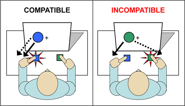
Source: Wildenberg et al. (2010)

Example: the Simon effect

Let’s import the data/simon.rda file¹. You can use the load() function or the read_rda().

simon <- read_rda(here("data", "simon.rda"))
head(simon)

#> # A tibble: 6 × 15
#>   submission_id    RT condition   correctness class    experiment_id key_pressed
#>           <dbl> <dbl> <chr>       <chr>       <chr>            <dbl> <chr>      
#> 1          7432  1239 incongruent correct     Intro C…            52 q          
#> 2          7432   938 incongruent correct     Intro C…            52 q          
#> 3          7432   744 incongruent correct     Intro C…            52 q          
#> 4          7432   528 incongruent correct     Intro C…            52 q          
#> 5          7432   706 incongruent correct     Intro C…            52 p          
#> 6          7432   547 congruent   correct     Intro C…            52 p          
#> # ℹ 8 more variables: p <chr>, pause <dbl>, q <chr>, target_object <chr>,
#> #   target_position <chr>, timeSpent <dbl>, trial_number <dbl>,
#> #   trial_type <chr>

1. Source: https://github.com/michael-franke/aida-package

Example: the Simon effect

For simplicity, let’s consider only a single subject (submission_id: 7432), otherwise the model require including random effects. We also exclude strange trials with RT > 2500 ms.

simon <- filter(simon, 
                submission_id == 7432,
                RT < 2500)

Example: the Simon effect

Let’s plot the reaction times. Clearly the two distributions are right-skewed with a difference in location (\(\mu\)). The shape also differs between thus also the skewness is probably different:

ggplot(simon, aes(x = RT, fill = condition)) +
  geom_density(alpha = 0.7)

Example: the Simon effect

Let’s see some summary statistics. We see the difference between the two conditions.

funs <- list(mean = mean, sd = sd, skew = psych::skew, cv = cv)
summ <- tapply(simon$RT, simon$condition, function(x) sapply(funs, function(f) f(x)))
summ

#> $congruent
#>        mean          sd        skew          cv 
#> 504.1818182  81.7038670   0.5328521   0.1620524 
#> 
#> $incongruent
#>        mean          sd        skew          cv 
#> 564.0312500 123.4188852   2.8702013   0.2188157

Example: the Simon effect

Given that we modelling the difference in \(\mu\), this is the expected difference. We are working on the log scale, thus the model is estimating the log difference or the log ratio.

summ$incongruent["mean"] - summ$congruent["mean"]
#>     mean 
#> 59.84943
log(summ$incongruent["mean"]) - log(summ$congruent["mean"])
#>      mean 
#> 0.1121727
log(summ$incongruent["mean"] / summ$congruent["mean"])
#>      mean 
#> 0.1121727

Example: the Simon effect

Let’s fit the model:

fit <- glm(RT ~ condition, data = simon, family = Gamma(link = "log"))
summary(fit)

#> 
#> Call:
#> glm(formula = RT ~ condition, family = Gamma(link = "log"), data = simon)
#> 
#> Coefficients:
#>                      Estimate Std. Error t value Pr(>|t|)    
#> (Intercept)           6.22294    0.02625 237.053  < 2e-16 ***
#> conditionincongruent  0.11217    0.03580   3.134  0.00218 ** 
#> ---
#> Signif. codes:  0 '***' 0.001 '**' 0.01 '*' 0.05 '.' 0.1 ' ' 1
#> 
#> (Dispersion parameter for Gamma family taken to be 0.03790215)
#> 
#>     Null deviance: 4.1148  on 118  degrees of freedom
#> Residual deviance: 3.7439  on 117  degrees of freedom
#> AIC: 1424.4
#> 
#> Number of Fisher Scoring iterations: 4

Example: the Simon effect

Plotting the results:

plot(ggeffect(fit))

Example: the Simon effect

The main parameter of interest here is the \(\beta_1\) representing the difference in \(\mu\). We can interpret \(\exp(\beta_1) = 1.119\) as the multiplicative increase in RT when moving from congruent to incongruent condition. In the RT scale, we have a difference of 59.8494318. Remember that the statistical test is performed on the link-function scale.

emmeans(fit, pairwise ~ condition)$contrast
#>  contrast                estimate     SE  df t.ratio p.value
#>  congruent - incongruent   -0.112 0.0358 117  -3.134  0.0022
#> 
#> Results are given on the log (not the response) scale.
emmeans(fit, pairwise ~ condition, type = "response")$contrast
#>  contrast                ratio    SE  df null t.ratio p.value
#>  congruent / incongruent 0.894 0.032 117    1  -3.134  0.0022
#> 
#> Tests are performed on the log scale

More about the Gamma distribution

I have written more notes about the intepretation of Gamma parameters especially for simulations:

https://filippogambarota.github.io/statnotes/understanding-gamma/understanding-gamma.html

References

Agresti, A. (2015). Foundations of linear and generalized linear models. John Wiley & Sons. https://play.google.com/store/books/details?id=jlIqBgAAQBAJ

Wildenberg, W. P. M. van den, Wylie, S. A., Forstmann, B. U., Burle, B., Hasbroucq, T., & Ridderinkhof, K. R. (2010). To head or to heed? Beyond the surface of selective action inhibition: A review. Frontiers in Human Neuroscience, 4, 222. https://doi.org/10.3389/fnhum.2010.00222