Generalized Linear Mixed-Effects Models

Author

Filippo Gambarota

Notation

\[ \mathbf{y}_{N \times 1} = \mathbf{X}_{N \times p} \boldsymbol{\beta}_{p \times 1} + \sum_{i=1}^{m} \mathbf{Z}_i^{(N \times q_i)} \mathbf{b}_i^{(q_i \times 1)} + \boldsymbol{\varepsilon}_{N \times 1} \]

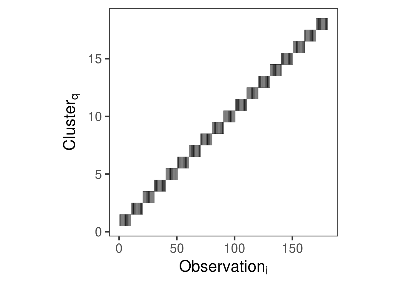
Where \(N\) is the number of observations, \(p\) is the number of predictors, \(q\) is the number of clusters (e.g., participants) and \(m\) is the number of random effects (e.g., nested or crossed).

Visualizing the \(\mathbf{Z}\) matrix

dat <- sleepstudy
Z <- get_Z_matrix(~ Days + (1|Subject), dat)
rownames(Z) <- NULL
colnames(Z) <- NULL

reshape2::melt(Z) |>
  ggplot(aes(x = Var1, y = Var2, fill = factor(value), color = factor(value))) +
  geom_tile(show.legend = FALSE) +
  scale_fill_manual(values = c("transparent", scales::alpha("black", 0.5))) +
  scale_color_manual(values = c("transparent", "black")) +
  theme_bw(20) +
  theme(panel.grid = element_blank(),
        aspect.ratio = 1) +
  ylab(latex2exp::TeX("$Cluster_q$")) +
  xlab(latex2exp::TeX("$Observation_i$"))

Why clustered data in Psychology?

In Psychology and Neuroscience we (almost) always have clustered data. For example:

Childrens nested within classrooms (maybe nested within schools)
Trials of a cognitive experiments nested within participants
…

The main point is that, clustered observations are not independent and we want to take into account the correlation.

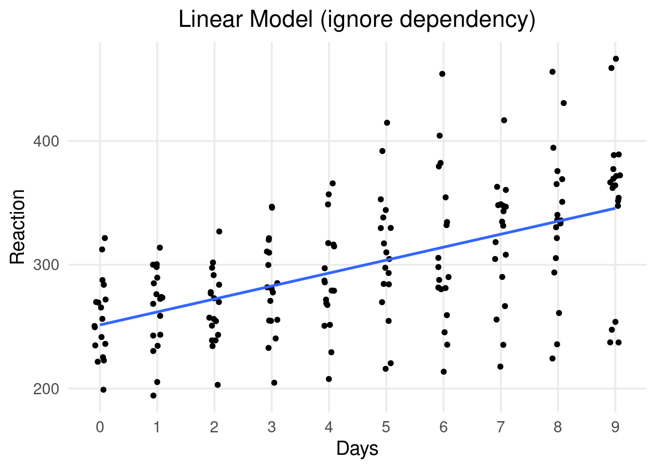
Example with `lme4::sleepstudy`

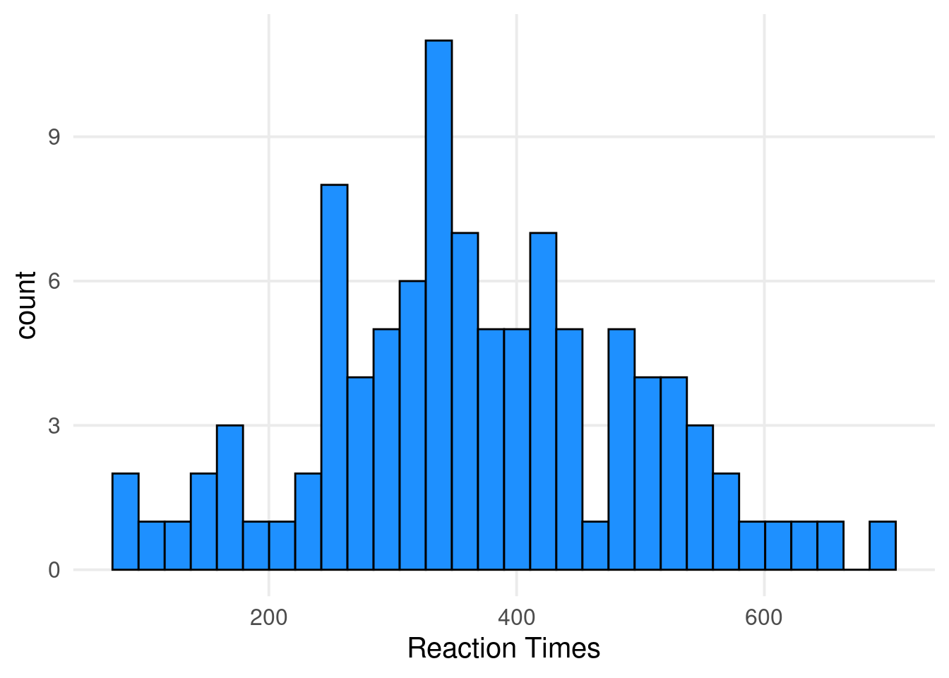
A very simple example is the lme4::sleepstudy where participants reaction times where evaluated under sleep deprivation.

dat <- lme4::sleepstudy
head(dat)

#>   Reaction Days Subject
#> 1 249.5600    0     308
#> 2 258.7047    1     308
#> 3 250.8006    2     308
#> 4 321.4398    3     308
#> 5 356.8519    4     308
#> 6 414.6901    5     308

Overall model

dat |> 
  ggplot(aes(x = Days, y = Reaction)) +
  geom_point(position = position_jitter(width = 0.1)) +
  scale_x_continuous(breaks = unique(dat$Days)) +
  geom_smooth(method = "lm", se = FALSE) +
  ggtitle("Linear Model (ignore dependency)")

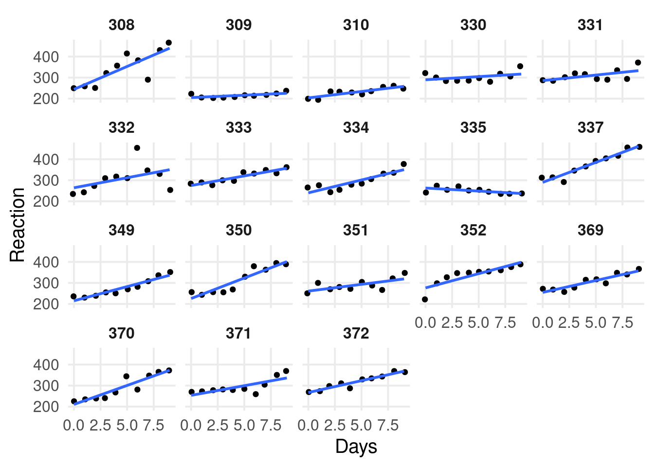
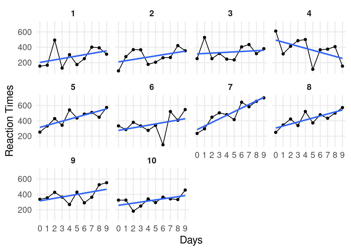
By-participant model

dat |> 
  ggplot(aes(x = Days, y = Reaction)) +
  geom_point(position = position_jitter(width = 0.1)) +
  facet_wrap(~Subject) +
  geom_smooth(method = "lm", se = FALSE)

By-participant model

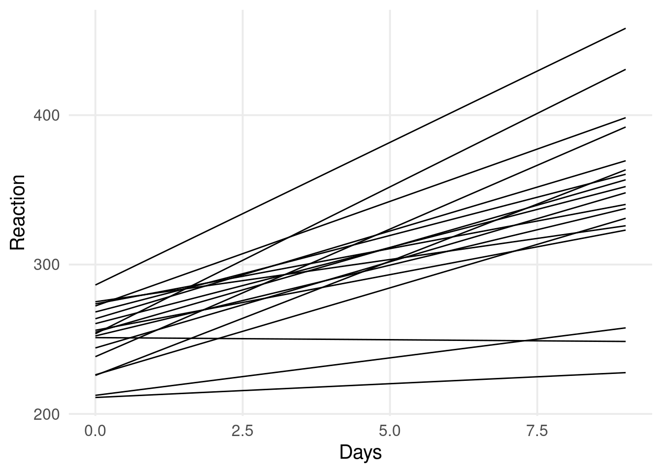
From the by-participant models, we see a clear dependency. Observations within the same participant are more similar compared to observations across participant.

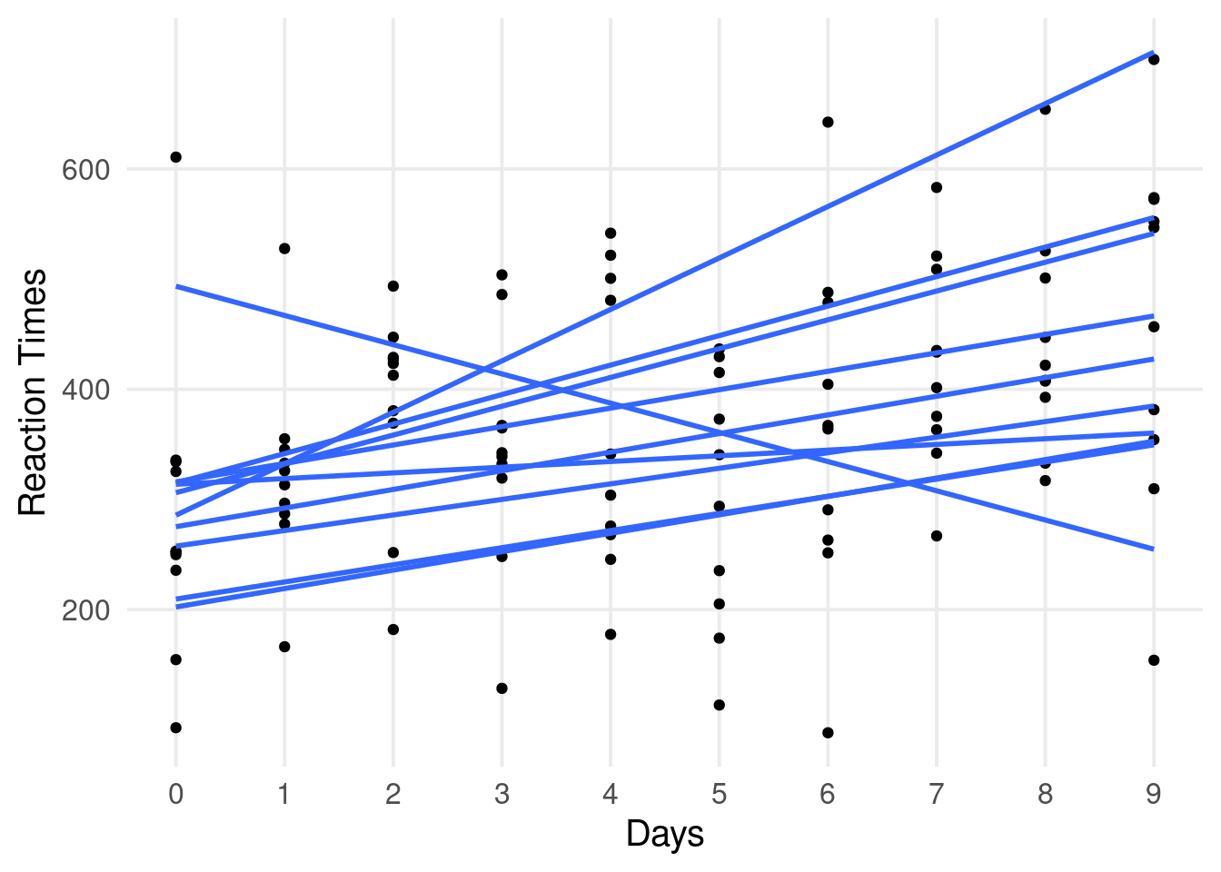
In addition, at Day 0, some participants have higher/lower reaction times compared to the overall trend. Similarly, some participants have higher/lower slopes.

Individual differences are the core of Psychology and we want to explictly model them!

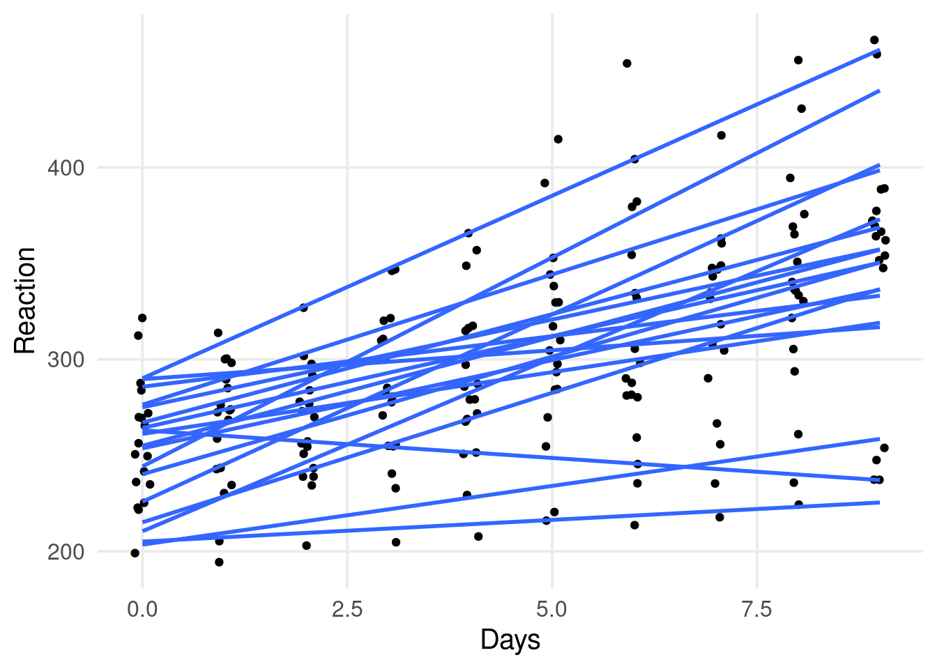
Individual differences

dat |> 
  ggplot(aes(x = Days, y = Reaction, group = Subject)) +
  geom_point(position = position_jitter(width = 0.1)) +
  geom_smooth(method = "lm", se = FALSE)

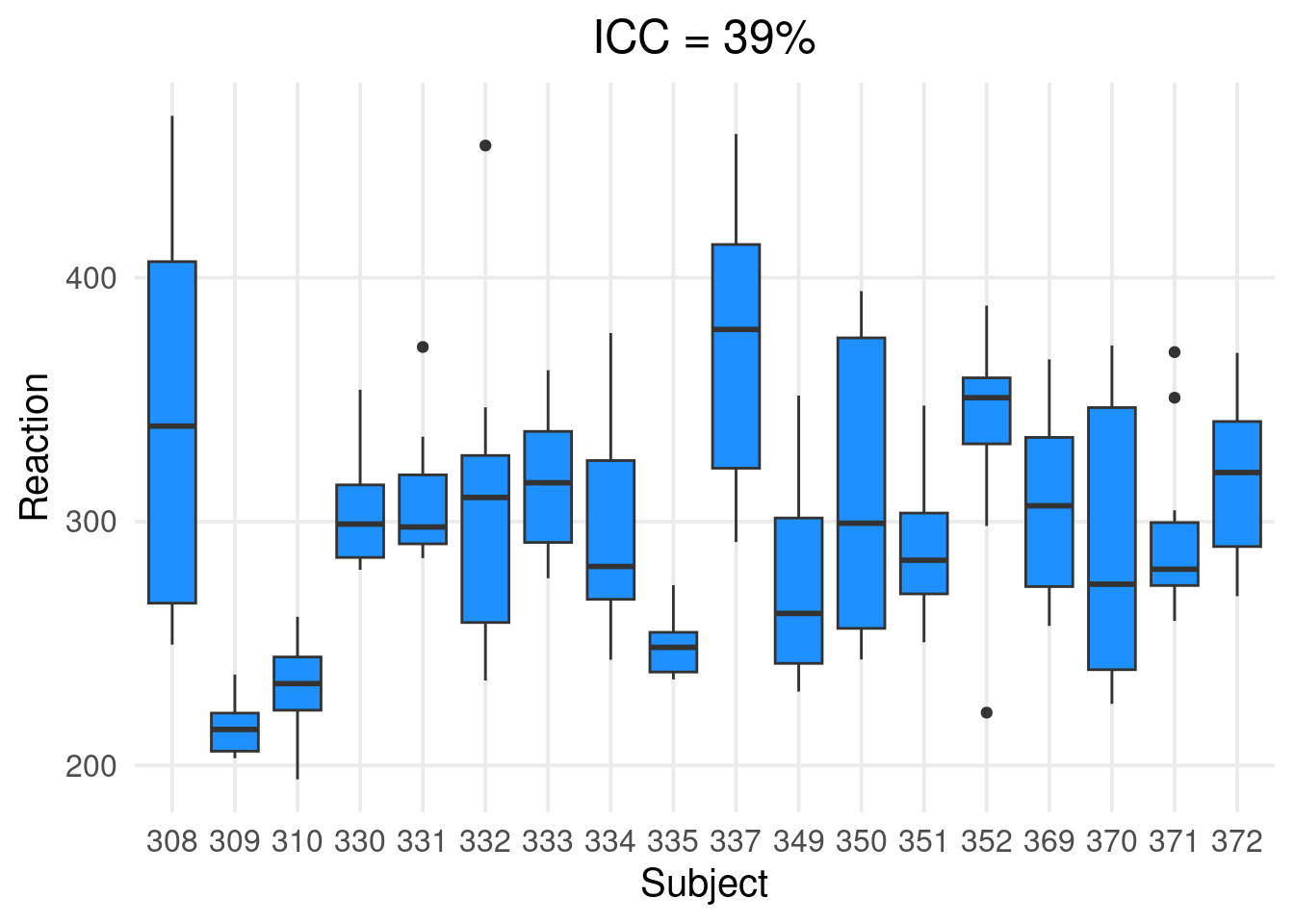
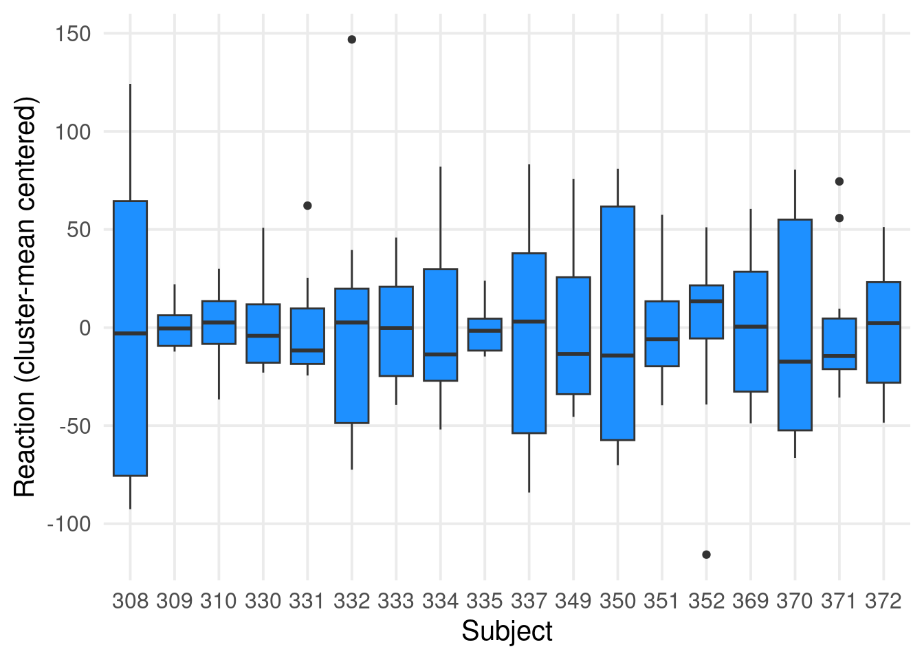
Are the observations clustered?

We can start assessing the clustering structure by fitting a mixed-model with only the random-intercepts and calculating the intraclass-correlation.

\[ y_{ij} = \beta_0 + \beta_{0_i} + \epsilon_{ij} \]

Are the observations clustered?

The model can be fitted with the lme4::lmer() function:

fit0 <- lmer(Reaction ~ 1 + (1|Subject), data = dat)
summary(fit0)

#> Linear mixed model fit by REML ['lmerMod']
#> Formula: Reaction ~ 1 + (1 | Subject)
#>    Data: dat
#> 
#> REML criterion at convergence: 1904.3
#> 
#> Scaled residuals: 
#>     Min      1Q  Median      3Q     Max 
#> -2.4983 -0.5501 -0.1476  0.5123  3.3446 
#> 
#> Random effects:
#>  Groups   Name        Variance Std.Dev.
#>  Subject  (Intercept) 1278     35.75   
#>  Residual             1959     44.26   
#> Number of obs: 180, groups:  Subject, 18
#> 
#> Fixed effects:
#>             Estimate Std. Error t value
#> (Intercept)   298.51       9.05   32.98

Are the observations clustered?

# using the insight::get_variance() function
vv <- insight::get_variance(fit0)
vv$var.intercept / (vv$var.intercept + vv$var.residual)

#>   Subject 
#> 0.3948896

# or directly with performance::icc()
performance::icc(fit0)

#> # Intraclass Correlation Coefficient
#> 
#>     Adjusted ICC: 0.395
#>   Unadjusted ICC: 0.395

Thus roughly 39% of the variance is explained by the clustering structure.

Are the observations clustered?

dat |> 
  ggplot(aes(x = Subject, y = Reaction)) +
  #geom_point(position = position_jitter(width = 0.1))
  geom_boxplot(fill = "dodgerblue") +
  ggtitle("ICC = 39%")

Are the observations clustered

We can remove the subject-specific effect.

dat |> 
  mutate(Reaction_cmc = cmc(Reaction, Subject)) |> 
  ggplot(aes(x = Subject, y = Reaction_cmc)) +
  #geom_point(position = position_jitter(width = 0.1))
  geom_boxplot(fill = "dodgerblue") +
  ylab("Reaction (cluster-mean centered)")

How different ICCs appear…

We can simulate some datasets with different ICC:

icc <- c(0, 0.3, 0.8)
sb0 <- sqrt(icc)

b0 <- 0

ns <- 10
nt <- 10

id <- rep(1:ns, each = nt)

y <- vector(mode = "list", length = length(icc))

for(i in 1:length(icc)){
  b0i <- rnorm(ns, 0, sb0[i])
  y[[i]] <- b0 + b0i[id] + rnorm(ns * nt, 0, 1 - sb0[i])
}

dd <- data.frame(
  id = rep(id, length(sb0)),
  sb0 = rep(sb0, each = ns * nt),
  icc = rep(icc, each = ns * nt),
  y = unlist(y)
)

dd |> 
  mutate(icc = sprintf("ICC = %s", icc),
         icc = factor(icc, levels = c("ICC = 0", "ICC = 0.3","ICC = 0.8"))) |> 
  ggplot(aes(x = factor(id), y = y)) +
  geom_boxplot() +
  facet_wrap(~icc) +
  xlab("Cluster")

Psychological interpretation of random intercepts

The random-intercepts are intepreted as baseline variation in the experiment. For example:

variability at time 0
variability pre treatment
variability for the reference condition
…

Furthemore, the ICC (that is related to the random-intercepts variance) affects the statistical power of the model.

Statistical power and ICC

We will see how to simulate data in a meaningful way, but here just an example on the impact of ICC on the statistical power.

I estimate the statistical power (for an intercept-only model) using the analytical method by Hedges and Pigott (2001).

powerICC <- function(nc, ns, d, icc, alpha = 0.05){
  tau2 <- icc
  vi <- 1/ns + 1/ns
  v <- (vi + tau2)/nc
  z <- d / sqrt(v)
  zc <- abs(qnorm(alpha/2))
  1 - pnorm(zc - z) + pnorm(-zc - z)
}

Statistical power and ICC

sim <- expand.grid(
  nc = c(1, seq(5, 50, 10)),
  ns = 20,
  d = 0.3,
  icc = c(0, 0.3, 0.5, 0.8)
) 

sim$power <- with(sim, powerICC(nc, ns, d, icc))

sim |> 
  ggplot(aes(x = icc, y = power, color = factor(nc))) +
  geom_line() +
  labs(color = "Clusters") +
  xlab("ICC") +
  ylab("Power") +
  ggtitle("N = 20 (per cluster), d = 0.3")

ICC in Psychology¹

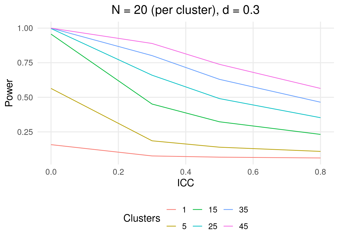
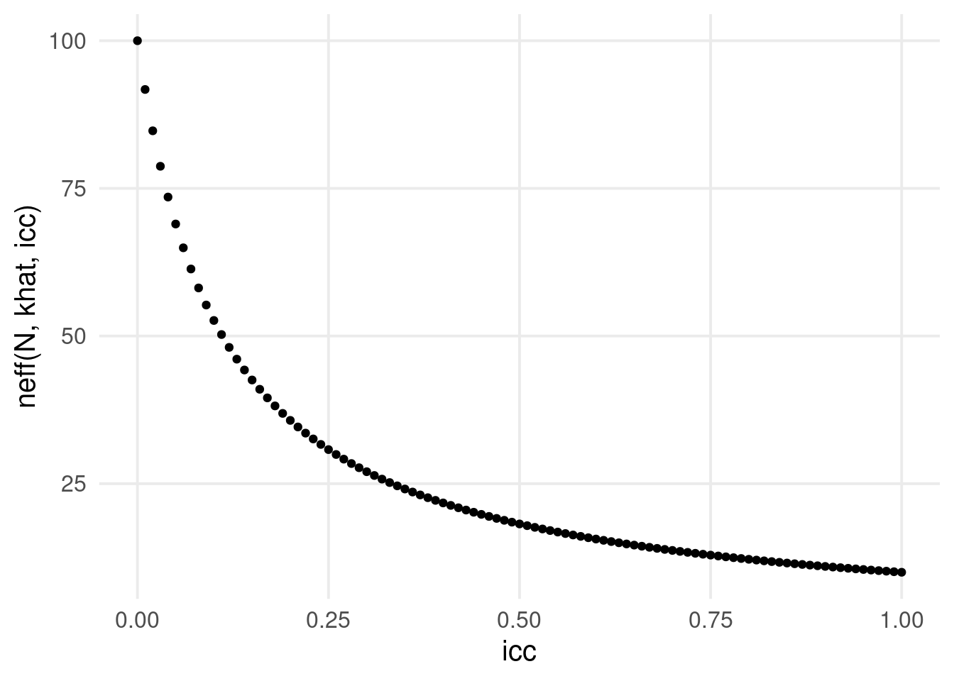
In Psychology it is common to collect clustered data and the data collection is usually time expensive. In addition, sample sizes are usually lower than the optimal level according to power calculation. Rao and Scott (1992) defined the concept of effective sample size for the reduction in the sample size (and thus power) according to the ICC in clustered data.

\[ N_{\text{eff}} = \frac{N}{1 + (\bar k - 1) \rho} \] Where \(\bar k\) is the average number of observations per cluster.

neff <- function(N, khat, icc){
  N / (1 + (khat - 1) * icc)
}

ICC in Psychology

N <- 100
khat <- 10
icc <- seq(0, 1, 0.01)

qplot(icc, neff(N, khat, icc), type = "l", lwd = 1)

Adding the fixed effect

Then we can add the fixed effect of Days. The variable is numeric starting with 0 up to 5 days. We can just add the variable as it is.

fit1 <- lmer(Reaction ~ Days + (1|Subject), data = dat)
# equivalent to
# fit1 <- update(fit0, . ~ . + Days)

summary(fit1)

#> Linear mixed model fit by REML ['lmerMod']
#> Formula: Reaction ~ Days + (1 | Subject)
#>    Data: dat
#> 
#> REML criterion at convergence: 1786.5
#> 
#> Scaled residuals: 
#>     Min      1Q  Median      3Q     Max 
#> -3.2257 -0.5529  0.0109  0.5188  4.2506 
#> 
#> Random effects:
#>  Groups   Name        Variance Std.Dev.
#>  Subject  (Intercept) 1378.2   37.12   
#>  Residual              960.5   30.99   
#> Number of obs: 180, groups:  Subject, 18
#> 
#> Fixed effects:
#>             Estimate Std. Error t value
#> (Intercept) 251.4051     9.7467   25.79
#> Days         10.4673     0.8042   13.02
#> 
#> Correlation of Fixed Effects:
#>      (Intr)
#> Days -0.371

Adding the fixed effect

This means that for each day we have an expected increase in reaction times of 10.47 milliseconds (or 0.01 seconds).

We have only the random intercept for subjects, thus we are assuming that each subject has the same sleep deprivation effect but can have different baseline reaction times.

head(coef(fit1)$Subject)

#>     (Intercept)     Days
#> 308    292.1888 10.46729
#> 309    173.5556 10.46729
#> 310    188.2965 10.46729
#> 330    255.8115 10.46729
#> 331    261.6213 10.46729
#> 332    259.6263 10.46729

# equivalent to fixef(fit1)["(Intercept)"] + ranef(fit1)$Subject for the random intercept

Adding the fixed effect

coef(fit1)$Subject |> 
  mutate(Subject = 1:n()) |> 
  mutate(b0 = fixef(fit1)[1],
         b1 = fixef(fit1)[2]) |> 
  rename("b0i" = `(Intercept)`,
         "b1i" = `Days`) |> 
  expand_grid(Days = unique(dat$Days)) |> 
  mutate(pi = b0i + b1i * Days,
         p = b0 + b1 * Days) |> 
  ggplot(aes(x = Days, y = pi)) +
  geom_line(aes(group = Subject),
            alpha = 0.5) +
  geom_line(aes(x = Days, y = p),
            lwd = 1.5,
            col = "firebrick") +
  ylab("Reaction")

Adding the fixed effect

coef(fit1)$Subject |> 
  mutate(Subject = 1:n()) |> 
  mutate(b0 = fixef(fit1)[1],
         b1 = fixef(fit1)[2]) |> 
  rename("b0i" = `(Intercept)`,
         "b1i" = `Days`) |> 
  expand_grid(Days = unique(dat$Days)) |> 
  mutate(pi = b0i + b1i * Days,
         p = b0 + b1 * Days) |> 
  ggplot(aes(x = Days, y = pi)) +
  geom_line(aes(group = Subject),
            alpha = 0.5) +
  geom_line(aes(x = Days, y = p),
            lwd = 1.5,
            col = "firebrick") +
  ylab("Reaction")

Adding the fixed effect

The same can be achieved using:

DD <- expand_grid(
  Subject = unique(dat$Subject),
  Days = unique(dat$Days)
)

DD$pi <- predict(fit1, newdata = DD)

head(DD)

#> # A tibble: 6 × 3
#>   Subject  Days    pi
#>   <fct>   <dbl> <dbl>
#> 1 308         0  292.
#> 2 308         1  303.
#> 3 308         2  313.
#> 4 308         3  324.
#> 5 308         4  334.
#> 6 308         5  345.

Is the fixed effect enough?

A big problem with mixed models is that effects can be included both as fixed and random and the choice is not always easy. From the plots at the beginning there is a clear variability in slopes that the model is ignoring.

fit2 <- lmer(Reaction ~ Days + (Days|Subject), data = dat)
summary(fit2)

#> Linear mixed model fit by REML ['lmerMod']
#> Formula: Reaction ~ Days + (Days | Subject)
#>    Data: dat
#> 
#> REML criterion at convergence: 1743.6
#> 
#> Scaled residuals: 
#>     Min      1Q  Median      3Q     Max 
#> -3.9536 -0.4634  0.0231  0.4634  5.1793 
#> 
#> Random effects:
#>  Groups   Name        Variance Std.Dev. Corr
#>  Subject  (Intercept) 612.10   24.741       
#>           Days         35.07    5.922   0.07
#>  Residual             654.94   25.592       
#> Number of obs: 180, groups:  Subject, 18
#> 
#> Fixed effects:
#>             Estimate Std. Error t value
#> (Intercept)  251.405      6.825  36.838
#> Days          10.467      1.546   6.771
#> 
#> Correlation of Fixed Effects:
#>      (Intr)
#> Days -0.138

Is the fixed effect enough?

The first important part is the estimation of the random part. Clearly the random slopes variance is not zero.

filter_output(summary(fit2), c("^Random effects|^Number of obs"))

#> Random effects:
#>  Groups   Name        Variance Std.Dev. Corr
#>  Subject  (Intercept) 612.10   24.741       
#>           Days         35.07    5.922   0.07
#>  Residual             654.94   25.592       
#> Number of obs: 180, groups:  Subject, 18

Is the fixed effect enough?

One of the most important part is that the standard error of the fixed coefficients is affected by the inclusion of the random slopes. Omitting the slopes was underestimating the standard error.

qualcosa su barr, keep it maximal, etc.

car::compareCoefs(fit1, fit2)

#> Calls:
#> 1: lmer(formula = Reaction ~ Days + (1 | Subject), data = dat)
#> 2: lmer(formula = Reaction ~ Days + (Days | Subject), data = dat)
#> 
#>             Model 1 Model 2
#> (Intercept)  251.41  251.41
#> SE             9.75    6.82
#>                            
#> Days         10.467  10.467
#> SE            0.804   1.546
#>

Is the fixed effect enough?

We can formally compare the models using a Likelihood Ratio Test (LRT)²:

anova(fit1, fit2)

#> Data: dat
#> Models:
#> fit1: Reaction ~ Days + (1 | Subject)
#> fit2: Reaction ~ Days + (Days | Subject)
#>      npar    AIC    BIC  logLik -2*log(L)  Chisq Df Pr(>Chisq)    
#> fit1    4 1802.1 1814.8 -897.04    1794.1                         
#> fit2    6 1763.9 1783.1 -875.97    1751.9 42.139  2  7.072e-10 ***
#> ---
#> Signif. codes:  0 '***' 0.001 '**' 0.01 '*' 0.05 '.' 0.1 ' ' 1

# or ranova(refitML(fit2))

Plotting the random slopes

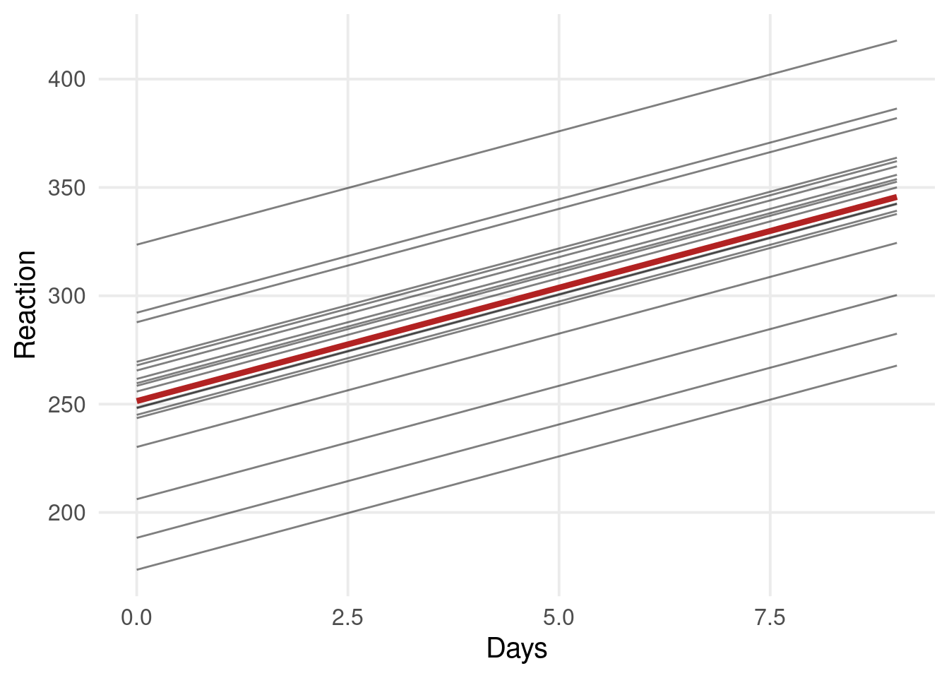
DD <- expand_grid(
  Subject = unique(dat$Subject),
  Days = unique(dat$Days)
)

DD$pi <- predict(fit2, newdata = DD)

DD |> 
  ggplot(aes(x = Days, y = pi, group = Subject)) +
  geom_line() +
  xlab("Days") +
  ylab("Reaction")

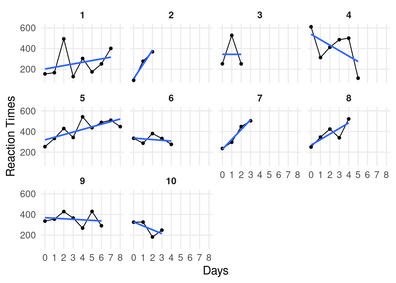
Shrinkage!

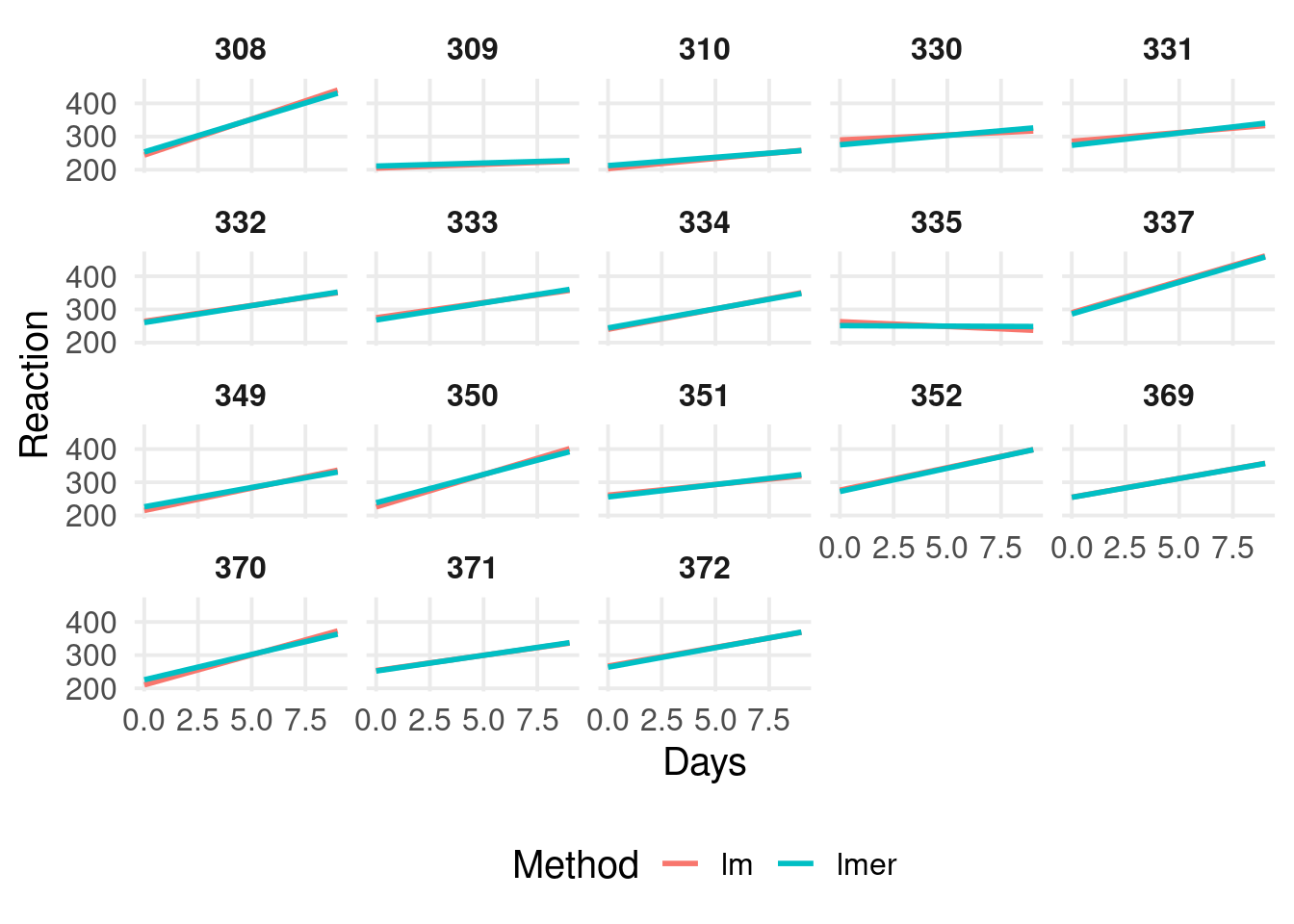
We can compare the fit of the multilevel model with linear models for each cluster. We can use the fit_by_cluster() function tha takes a formula, a grouping factor and fit a model for each cluster.

fitl <- fit_by_cluster(Reaction ~ Days | Subject,
                       dat,
                       model = lm)

Shrinkage!

fitl <- fit_by_cluster(Reaction ~ Days | Subject,
                       dat,
                       model = lm)

DD <- expand_grid(
  Subject = unique(dat$Subject),
  Days = unique(dat$Days)
)

DD$lmer <- predict(fit2, DD)
DD$Subject <- as.numeric(as.character(DD$Subject))

subjs <- unique(DD$Subject)
DD$lm <- NA

for(i in 1:length(fitl)){
  pp <- predict(fitl[[i]], DD[DD$Subject == subjs[i], ])
  DD$lm[DD$Subject == subjs[i]] <- pp
}

DD |> 
  pivot_longer(c(lmer, lm)) |> 
  ggplot(aes(x = Days, y = value, color = name)) +
  geom_line(lwd = 1) +
  facet_wrap(~Subject) +
  ylab("Reaction") +
  labs(color = "Method")

Let’s simulate a multilevel model!

Let’s try to simulate the previous model

N <- 10
DAYS <- 10 # max number of days
b00 <- 300 # grand-mean of reaction times at time 0
b1 <- 20  # increase in reaction time for each day
sb0 <- 30 # standard deviation intercepts
sb1 <- 10 # standard deviaton slopes
s <- 100 # residual standard deviation

# we are simulating an ICC of
sb0^2 / (sb0^2 + s^2)
#> [1] 0.08256881

sim <- expand_grid(
  id = 1:N,
  days = 0:(DAYS - 1)
)

# random intercepts and slopes, rho = 0

R <- 0 + diag(1 - 0, 2)
VCOV <- diag(c(sb0, sb1)) %*% R %*% diag(c(sb0, sb1))

RE <- MASS::mvrnorm(N, c(0, 0), VCOV)

b0i <- RE[, 1]
b1i <- RE[, 2]

# linear predictor
sim$lp <- with(sim, b00 + b0i[id] + (b1 + b1i[id]) * days)
sim$rt <- rnorm(nrow(sim), sim$lp, s)

Let’s try to simulate the previous model

sim |> 
  ggplot(aes(x = rt)) +
  geom_histogram(color = "black",
                 fill = "dodgerblue") +
  xlab("Reaction Times")

Let’s try to simulate the previous model

sim |> 
  ggplot(aes(x = days, y = rt)) +
  geom_point() +
  scale_x_continuous(breaks = 0:DAYS) +
  xlab("Days") +
  ylab("Reaction Times") +
  geom_smooth(method = "lm",
              se = FALSE,
              aes(group = id))

Let’s try to simulate the previous model

sim |> 
  ggplot(aes(x = days, y = rt)) +
  geom_point() +
  geom_line() +
  scale_x_continuous(breaks = 0:DAYS) +
  xlab("Days") +
  ylab("Reaction Times") +
  facet_wrap(~id, ncol = 4) +
  geom_smooth(method = "lm",
              se = FALSE)

Let’s try to simulate the previous model

A more realistic scenario could be to have an heterogeneous number of observations for each cluster.

# minimum 3 observations
ndays_per_subject <- sample(3:(DAYS - 1), size = N, replace = TRUE)
siml <- split(sim, sim$id)

for(i in 1:length(siml)){
  siml[[i]] <- siml[[i]][1:ndays_per_subject[i], ]
}

sim_missing <- do.call(rbind, siml)

# number of observations
tapply(sim_missing$rt, sim_missing$id, length)
#>  1  2  3  4  5  6  7  8  9 10 
#>  8  3  3  6  9  5  4  5  7  4

Let’s try to simulate the previous model

sim_missing |> 
  ggplot(aes(x = days, y = rt)) +
  geom_point() +
  geom_line() +
  scale_x_continuous(breaks = 0:DAYS) +
  xlab("Days") +
  ylab("Reaction Times") +
  facet_wrap(~id, ncol = 4) +
  geom_smooth(method = "lm",
              se = FALSE)

Let’s fit the model

Here the random-intercepts and slopes model:

fit <- lmer(rt ~ days + (days|id), data = sim_missing)
summary(fit)

#> Linear mixed model fit by REML ['lmerMod']
#> Formula: rt ~ days + (days | id)
#>    Data: sim_missing
#> 
#> REML criterion at convergence: 650
#> 
#> Scaled residuals: 
#>      Min       1Q   Median       3Q      Max 
#> -2.10251 -0.66077  0.00732  0.63516  2.01985 
#> 
#> Random effects:
#>  Groups   Name        Variance Std.Dev. Corr 
#>  id       (Intercept)  3543.5   59.53        
#>           days          451.5   21.25   -0.77
#>  Residual             10994.3  104.85        
#> Number of obs: 54, groups:  id, 10
#> 
#> Fixed effects:
#>             Estimate Std. Error t value
#> (Intercept)   313.18      30.20  10.369
#> days           12.14      11.03   1.101
#> 
#> Correlation of Fixed Effects:
#>      (Intr)
#> days -0.761

Can the multilevel model be misleading?

What do you see in this plot?

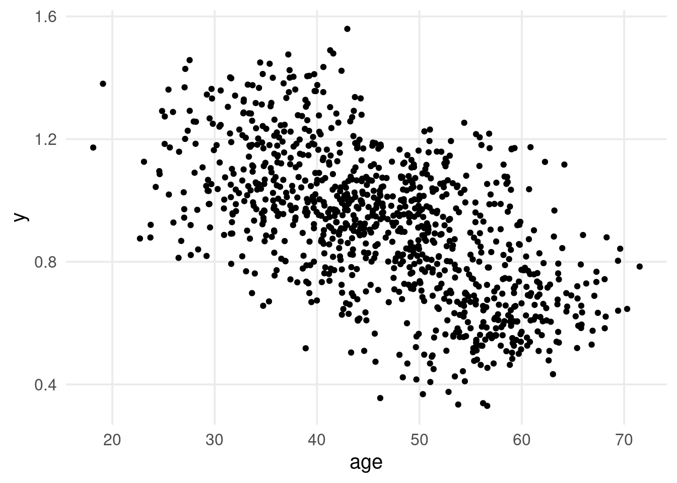
k <- 10 # number of clusters/units
n <- 100 # number of participants within each unit
N <- n * k # total sample size
unit <- rep(1:k, each = n)

age <- rnorm(N, 60 - 3 * (unit - 1), 5) # age equation
y <- 0 + rnorm(k, 0, 0.1)[unit] + 0.01 * age + 0.1 * (unit-1) + rnorm(N, 0, 0.1) # response equation
dat <- data.frame(unit, age, y)

dat |> 
  ggplot(aes(x = age, y = y)) +
  geom_point()

. . .

There is a clear negative relationship between age and the response variable y!

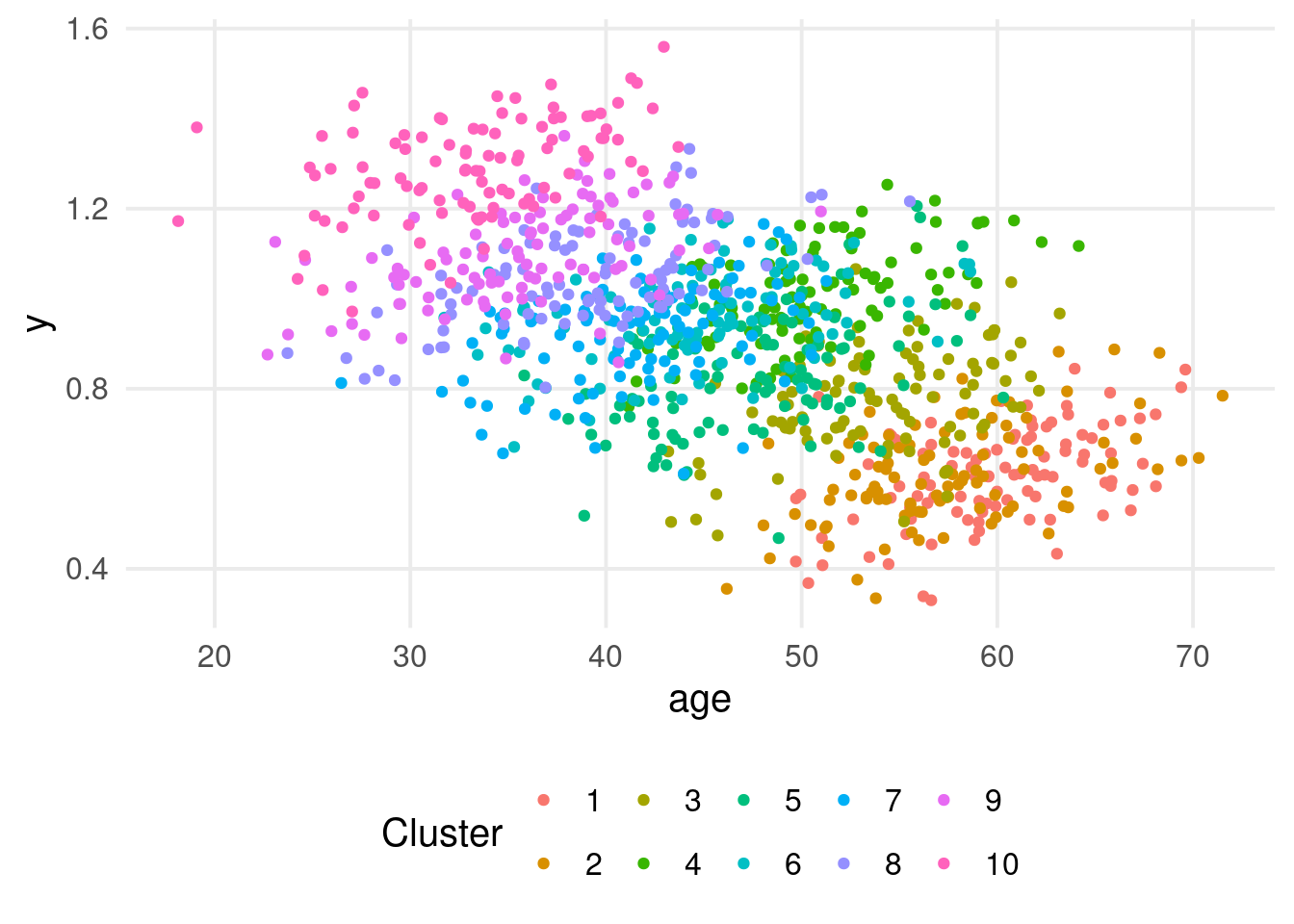
What do you see in this plot?

Let’s add the cluster information. What about now?

dat |> 
  ggplot(aes(x = age, y = y)) +
  geom_point(aes(color = factor(unit))) +
  labs(color = "Cluster")

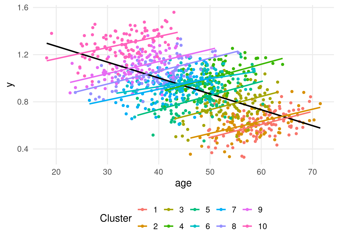
Simpson’s paradox

We have clustered data, and the relationship y ~ age seems to be different within and between clusters.
This phenomenon is called Simpson’s paradox and can be a serious problem in multilevel models.
Clearly this is a problem only for variables at the observation level (not at the cluster level).
For example, if clusters are schools and the observations are children. age is a variable at the children level (or aggregated at the school level). On the other side, the prestige of the school is a variable at the school level (the same for each child)

Simpson’s paradox

dat |> 
  ggplot(aes(x = age, y = y)) +
  geom_point(aes(color = factor(unit))) +
  labs(color = "Cluster") + 
  geom_smooth(method = "lm",
              se = FALSE,
              col = "black") +
  geom_smooth(method = "lm",
              aes(group = unit,
                  color = factor(unit)),
              se = FALSE)

Simpson’s paradox, what to do?

The main strategy to deal with the Simpson’s paradox is centering the variables. Enders and Tofighi (2007) provide a clear overview of the strategy.

Simpson’s paradox, what to do?

We can define some centering functions and see how we can model the multilevel structure.

filor::print_fun(c(funs$cm, funs$cmc, funs$gmc))

cm <- function(x, cluster){
  cm <- tapply(x, cluster, mean)
  cm[cluster]
}
cmc <- function(x, cluster){
  x - cm(x, cluster)
}
gmc <- function(x){
  x - mean(x)
}

Simpson’s paradox, between-clusters effect

Firsly we can calculate the clusters mean. This remove the within-effect and a linear model will capture only the between-effect.

dat |> 
  mutate(age_cm = cm(age, unit),
         y_cm = cm(y, unit)) |> 
  ggplot(aes(x = age, y = y)) +
  geom_point(alpha = 0.2,
             aes(color = factor(unit))) +
  geom_point(aes(x = age_cm, y = y_cm,
                 color = factor(unit)),
             alpha = 1,
             size = 4) +
  labs(color = "Unit")

Simpson’s paradox, between-clusters effect

We have a negative age effect between clusters, as expected.

dat_cm <- dat |> 
  group_by(unit) |> 
  summarise(y_cm = mean(y),
            age_cm = mean(age))

lm(y_cm ~ age_cm, data = dat_cm)

#> 
#> Call:
#> lm(formula = y_cm ~ age_cm, data = dat_cm)
#> 
#> Coefficients:
#> (Intercept)       age_cm  
#>     1.92527     -0.02175

Simpson’s paradox, within-clusters effect

We can substract (i.e., centering) from each observation, the cluster mean.

dat |> 
  mutate(age_cm = cm(age, unit),
         age_cmc = cmc(age, unit),
         y_cm = cm(y, unit)) |> 
  ggplot(aes(x = age_cmc, y = y)) +
  geom_point(alpha = 0.2,
             aes(color = factor(unit))) +
  xlab(latex2exp::TeX("$age - \\; \\bar{age_k}$")) +
  geom_point(aes(x = 0, y = y_cm,
                 color = factor(unit))) +
  geom_smooth(method = "lm",
              aes(group = unit,
                  color = factor(unit)),
              se = FALSE) +
  labs(color = "Unit")

Simpson’s paradox, within-clusters effect

dat$age_cmc <- cmc(dat$age, dat$unit)

fitl_cmc <- fit_by_cluster(
  y ~ age_cmc | unit,
  data = dat,
  model = lm
)

Simpson’s paradox, within-clusters effect

All slopes are similar but positive (compared to the between-effect). Thus estimating only the between (or within) effect is completely misleading.

fitl_cmc |> 
  lapply(broom::tidy, conf.int = TRUE) |> 
  bind_rows(.id = "unit") |> 
  mutate(unit = as.numeric(unit)) |> 
  filter(term == "age_cmc") |> 
  ggplot(aes(x = estimate, y = unit)) +
  geom_pointrange(aes(xmin = conf.low, xmax = conf.high)) +
  geom_vline(xintercept = 0,
             lty = "dashed",
             col = "firebrick") +
  xlab(latex2exp::TeX("$\\beta_{age}$"))

What about the multilevel model?

We can fit a multilevel model on the full dataset. What is the age slope? within or between?

fit <- lmer(y ~ age + (1|unit), data = dat)
summary(fit)

#> Linear mixed model fit by REML ['lmerMod']
#> Formula: y ~ age + (1 | unit)
#>    Data: dat
#> 
#> REML criterion at convergence: -1710.7
#> 
#> Scaled residuals: 
#>     Min      1Q  Median      3Q     Max 
#> -3.7439 -0.6848 -0.0165  0.7191  3.0376 
#> 
#> Random effects:
#>  Groups   Name        Variance Std.Dev.
#>  unit     (Intercept) 0.091429 0.30237 
#>  Residual             0.009747 0.09872 
#> Number of obs: 1000, groups:  unit, 10
#> 
#> Fixed effects:
#>              Estimate Std. Error t value
#> (Intercept) 0.4471843  0.0997411   4.483
#> age         0.0100761  0.0006074  16.590
#> 
#> Correlation of Fixed Effects:
#>     (Intr)
#> age -0.283

What about the multilevel model?

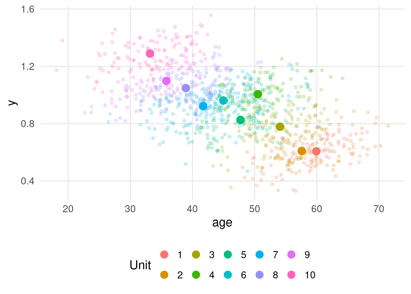
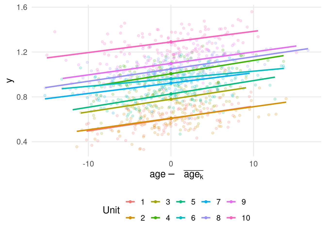
The estimated effect is a sort of weighted average of the within and between effect. This is usually not interesting, especially when the two effects are different. We want to isolate the between and within effects.

We need to include two version of the age variable, one centered on the clusters and the other representing the clusters means.

dat$age_cmc <- cmc(dat$age, dat$unit)
dat$age_cm <- cm(dat$age, dat$unit)

fit_bw <- lmer(y ~ age_cmc + age_cm + (1|unit), data = dat)

What about the multilevel model?

summary(fit_bw)

#> Linear mixed model fit by REML ['lmerMod']
#> Formula: y ~ age_cmc + age_cm + (1 | unit)
#>    Data: dat
#> 
#> REML criterion at convergence: -1724.4
#> 
#> Scaled residuals: 
#>     Min      1Q  Median      3Q     Max 
#> -3.7518 -0.6848 -0.0136  0.7126  3.0452 
#> 
#> Random effects:
#>  Groups   Name        Variance Std.Dev.
#>  unit     (Intercept) 0.007530 0.08678 
#>  Residual             0.009746 0.09872 
#> Number of obs: 1000, groups:  unit, 10
#> 
#> Fixed effects:
#>               Estimate Std. Error t value
#> (Intercept)  1.9252710  0.1503998  12.801
#> age_cmc      0.0101730  0.0006083  16.724
#> age_cm      -0.0217498  0.0031833  -6.832
#> 
#> Correlation of Fixed Effects:
#>         (Intr) ag_cmc
#> age_cmc  0.000       
#> age_cm  -0.983  0.000

What about the multilevel model?

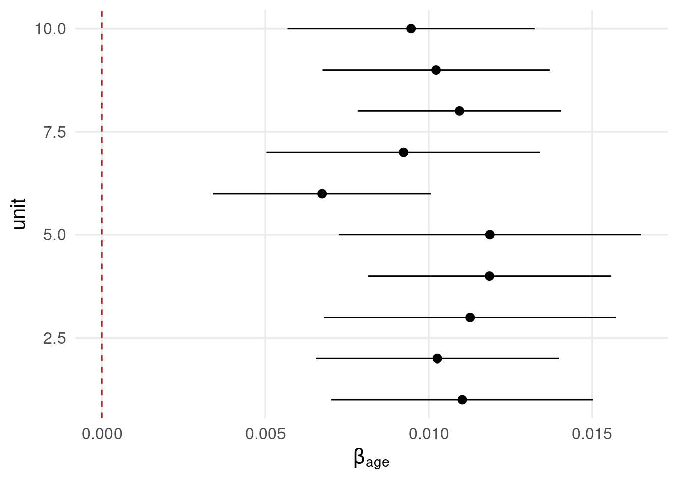
The within-clusters effect can be also included as random slope³. Basically we allows not only the within effect to be different compared to the between effect but also that each cluster has a different sloope.

fit_bw2 <- lmer(y ~ age_cmc + age_cm + (age_cmc|unit), data = dat)
summary(fit_bw2)

#> Linear mixed model fit by REML ['lmerMod']
#> Formula: y ~ age_cmc + age_cm + (age_cmc | unit)
#>    Data: dat
#> 
#> REML criterion at convergence: -1724.5
#> 
#> Scaled residuals: 
#>     Min      1Q  Median      3Q     Max 
#> -3.7516 -0.6911 -0.0114  0.7116  3.0458 
#> 
#> Random effects:
#>  Groups   Name        Variance  Std.Dev.  Corr
#>  unit     (Intercept) 7.528e-03 0.0867634     
#>           age_cmc     2.053e-08 0.0001433 1.00
#>  Residual             9.746e-03 0.0987213     
#> Number of obs: 1000, groups:  unit, 10
#> 
#> Fixed effects:
#>              Estimate Std. Error t value
#> (Intercept)  1.933188   0.149989  12.889
#> age_cmc      0.010176   0.000610  16.683
#> age_cm      -0.021920   0.003174  -6.905
#> 
#> Correlation of Fixed Effects:
#>         (Intr) ag_cmc
#> age_cmc  0.020       
#> age_cm  -0.983 -0.006
#> optimizer (nloptwrap) convergence code: 0 (OK)
#> boundary (singular) fit: see help('isSingular')

More on the Simpson’s Paradox

Kievit et al. (2013) describe the SP problem in Psychology with methods to detect it.

What do you think?

Practical session

simulate clustered data with some predictors
simulate the same dataset but with a some between-within differences

Diagnostics

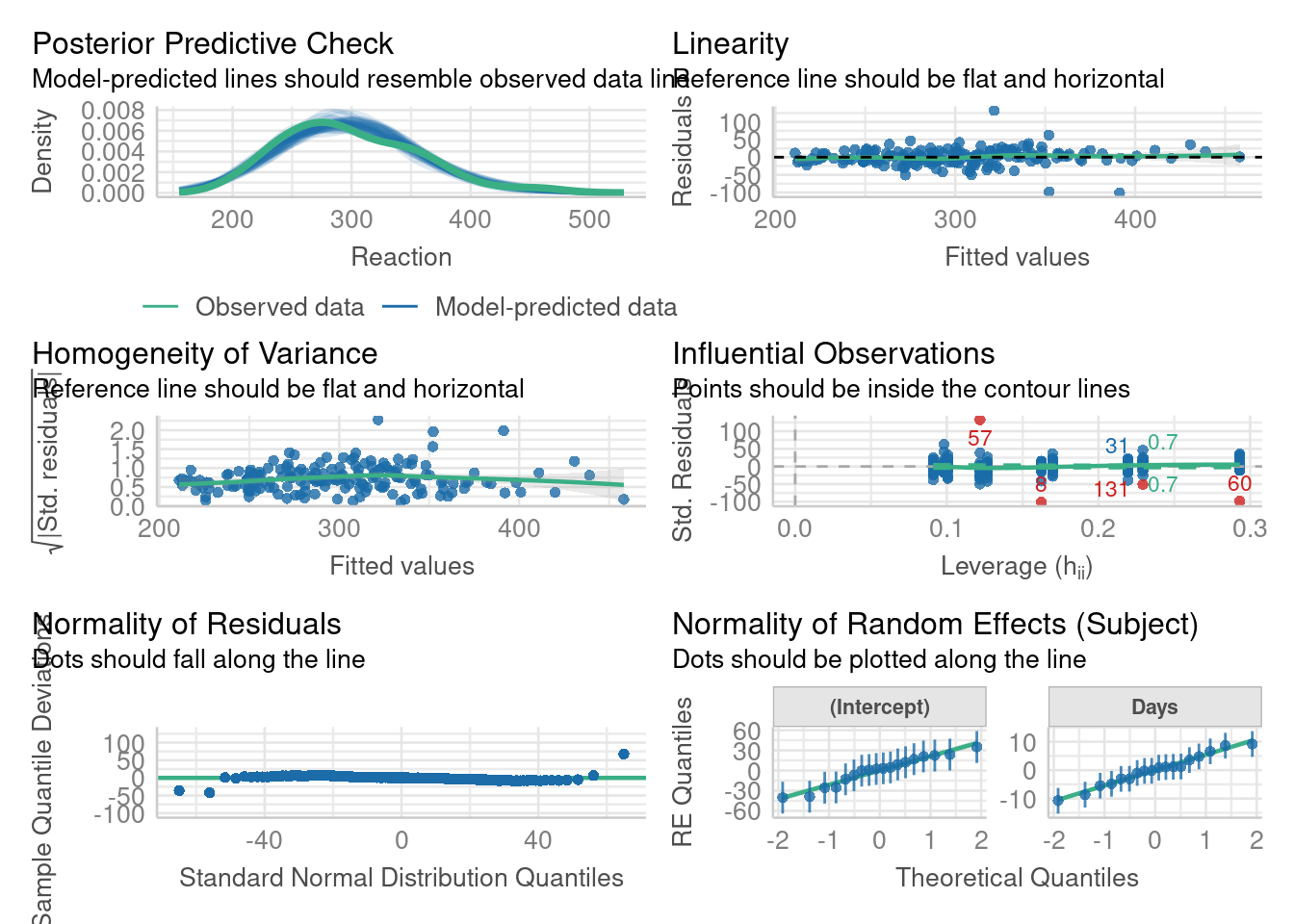
The `performance` package

The performance package has a series of nice functions to visualize and assess the models fit.

Let’s go back to our reaction times:

fit <- lmer(Reaction ~ Days + (Days|Subject), data = sleepstudy)

performance::check_model(fit)

The `performance` package

fit <- lmer(Reaction ~ Days + (Days|Subject), data = sleepstudy)

performance::check_model(fit)

Influence measures

Nieuwenhuis et al. (2012) describe the Influence.ME package that computes the standard influence measures (Cook’s distance, DFbeta, etc.) for lme4 models.

Also the lme4:::influence.merMod() compute all the measures. You can provide the groups = argument to specify at which level performing the leave-one-out procedure.

Influence measures, small exercise

Both lme4:::influence.merMod() and Influence.ME do not provide (good enough) plotting tools. Write a set of functions that takes a lme4 model in input, calculate the influence measures, organize everything in a data.frame and plot the influence measures results with ggplot2.

Effect sizes

\(R^2\) for multilevel models

The \(R^2\) for multilevel models is not computed as for standard regression models. Nakagawa, Johnson, and Schielzeth (2017) describe how to calculate the \(R^2\). They described the marginal (only fixed-effects) and the conditional (fixed and random-effects).

# or performance::r2()
performance::r2_nakagawa(fit)

#> # R2 for Mixed Models
#> 
#>   Conditional R2: 0.799
#>      Marginal R2: 0.279

Clearly the conditional is always greater or equal to the marginal one.

References

Enders, Craig K, and Davood Tofighi. 2007. “Centering Predictor Variables in Cross-Sectional Multilevel Models: A New Look at an Old Issue.” Psychological Methods 12 (June): 121–38. https://doi.org/10.1037/1082-989X.12.2.121.

Hedges, L V, and T D Pigott. 2001. “The Power of Statistical Tests in Meta-Analysis.” Psychological Methods 6 (September): 203–17. https://www.ncbi.nlm.nih.gov/pubmed/11570228.

Kievit, Rogier A, Willem E Frankenhuis, Lourens J Waldorp, and Denny Borsboom. 2013. “Simpson’s Paradox in Psychological Science: A Practical Guide.” Frontiers in Psychology 4 (August): 513. https://doi.org/10.3389/fpsyg.2013.00513.

Nakagawa, Shinichi, Paul C D Johnson, and Holger Schielzeth. 2017. “The Coefficient of Determination R2 and Intra-Class Correlation Coefficient from Generalized Linear Mixed-Effects Models Revisited and Expanded.” Journal of the Royal Society, Interface / the Royal Society 14 (September). https://doi.org/10.1098/rsif.2017.0213.

Nieuwenhuis, Rense, Manfred, Te Grotenhuis, and Ben Pelzer. 2012. “Influence.ME: Tools for Detecting Influential Data in Mixed Effects Models.” The R Journal 4: 38. https://doi.org/10.32614/rj-2012-011.

Rao, J N, and A J Scott. 1992. “A Simple Method for the Analysis of Clustered Binary Data.” Biometrics 48 (June): 577–85. https://doi.org/10.2307/2532311.

Footnotes

This is just an approximation to estimate the impact of the ICC↩︎
Note that the anova() function is refitting models using Maximum Likelihood (and not REML). This is required to compare models using LRT↩︎
Of course, including the clusters means as random-slopes is not possible. Note that data are simulated without random slopes, thus the model estimate parameters at the boundaries↩︎

Notation

Visualizing the \(\mathbf{Z}\) matrix

Why clustered data in Psychology?

Example with lme4::sleepstudy

Overall model

By-participant model

By-participant model

Individual differences

Are the observations clustered?

Are the observations clustered?

Are the observations clustered?

Are the observations clustered?

Are the observations clustered

How different ICCs appear…

Psychological interpretation of random intercepts

Statistical power and ICC

Statistical power and ICC

ICC in Psychology1

ICC in Psychology

Adding the fixed effect

Adding the fixed effect

Adding the fixed effect

Adding the fixed effect

Adding the fixed effect

Is the fixed effect enough?

Is the fixed effect enough?

Is the fixed effect enough?

Is the fixed effect enough?

Plotting the random slopes

Shrinkage!

Shrinkage!

Let’s simulate a multilevel model!

Let’s try to simulate the previous model

Let’s try to simulate the previous model

Let’s try to simulate the previous model

Let’s try to simulate the previous model

Let’s try to simulate the previous model

Let’s try to simulate the previous model

Let’s fit the model

Can the multilevel model be misleading?

What do you see in this plot?

What do you see in this plot?

Simpson’s paradox

Simpson’s paradox

Simpson’s paradox, what to do?

Simpson’s paradox, what to do?

Simpson’s paradox, between-clusters effect

Simpson’s paradox, between-clusters effect

Simpson’s paradox, within-clusters effect

Simpson’s paradox, within-clusters effect

Simpson’s paradox, within-clusters effect

What about the multilevel model?

What about the multilevel model?

What about the multilevel model?

What about the multilevel model?

More on the Simpson’s Paradox

Practical session

Diagnostics

The performance package

The performance package

Influence measures

Influence measures, small exercise

Effect sizes

\(R^2\) for multilevel models

References

Footnotes

Example with `lme4::sleepstudy`

ICC in Psychology¹

The `performance` package

The `performance` package