Multilevel and Multivariate Meta-analysis

Author

Filippo Gambarota

Quick recap of the two-level model

What we did so far about the two-level model (fixed/equal or random) is combining primary studies summarising each study with an effect size and precision measure.

From https://bookdown.org/MathiasHarrer/Doing_Meta_Analysis_in_R/multilevel-ma.html

In this model, effect sizes (and variances) are considered independent because they are collected on different participants. In other terms each row of a meta-analysis dataset is assumed independent.

In this example from the dat.bcg dataset (?dat.bcg) each row comes from a different study with different participants.

### calculate log risk ratios and corresponding sampling variances
dat <- escalc(measure="RR", ai=tpos, bi=tneg, ci=cpos, di=cneg, data=dat.bcg)
head(dat)

  trial               author year tpos  tneg cpos  cneg ablat     alloc      yi 
1     1              Aronson 1948    4   119   11   128    44    random -0.8893 
2     2     Ferguson & Simes 1949    6   300   29   274    55    random -1.5854 
3     3      Rosenthal et al 1960    3   228   11   209    42    random -1.3481 
4     4    Hart & Sutherland 1977   62 13536  248 12619    52    random -1.4416 
5     5 Frimodt-Moller et al 1973   33  5036   47  5761    13 alternate -0.2175 
6     6      Stein & Aronson 1953  180  1361  372  1079    44 alternate -0.7861 
      vi 
1 0.3256 
2 0.1946 
3 0.4154 
4 0.0200 
5 0.0512 
6 0.0069 

More formally, the two-level random-effects model can be written as:

\[ y_i = \mu_{\theta} + \delta_i + \epsilon_i \]

\[ \delta_i \sim \mathcal{N}(0, \tau^2) \]

\[ \epsilon_i \sim \mathcal{N}(0, \sigma^2_{\epsilon_i}) \]

Dependency

There are situations where effect sizes (and variances) are no longer independent. There are mainly two sources of dependency:

  1. multiple effect sizes within the same paper but with different participants
  2. multiple effect sizes collected on the same pool of participants

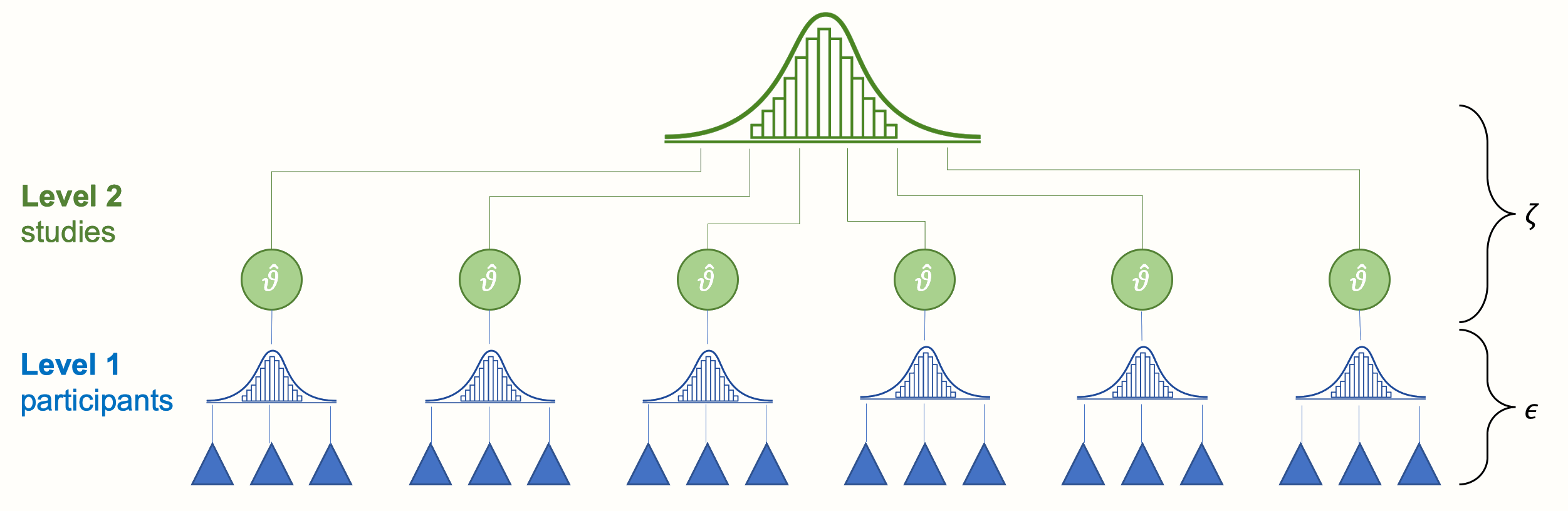
The first case refer to a situation where the effect sizes are nested within a paper and given that they will share a similar methodology, same authors, etc. they are likely more similar to each other compared to effect sizes from different papers. We can call this situation a multilevel dataset.

In the second case, the effects are correlated because they are collected on the same pool of participants thus sampling errors are correlated. This is the case where multiple outcome measures are collected or multiple time-points (like a longitudinal design). We can call this situation a multivariate dataset.

Importantly, the two type of meta-analysis will be very similar both formally and from the R implementation point of view but they are clearly distincted from an empirical point of view.

Multilevel meta-analysis

The multilevel data structure can be easily depicted in the figure below.

From https://bookdown.org/MathiasHarrer/Doing_Meta_Analysis_in_R/multilevel-ma.html

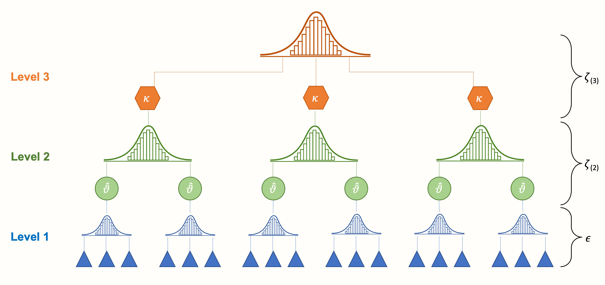
Also this picture clearly show the data structure and important parameters:

We can have several levels beyond the two-level model but usually common meta-analyses have a maximum of 3-4 levels. For example, it is common in experimental Psychology to have papers with more than one experiment with different participants.

More formally, a three-level model can be written as:

\[\begin{align} \begin{gathered} y_{ij} = \mu_{\theta} + \delta_i + \zeta_{ij} + \epsilon_{ij} \end{gathered} \end{align}\]

\[\begin{align} \begin{gathered} \delta_i\sim \mathcal{N}(0, \tau^2) \end{gathered} \end{align}\]

\[\begin{align} \begin{gathered} \zeta_{ij} \sim \mathcal{N}(0, \omega^2) \end{gathered} \end{align}\]

\[\begin{align} \begin{gathered} \epsilon_{ij} \sim \mathcal{N}(0,\sigma_{\epsilon_{ij}}^{2}) \end{gathered} \end{align}\]

The only addition is an extra source of heterogeneity \(\omega^2\) that can be intepreted as the true heterogeneity between effects nested within the same paper (or whatever is the cluster).

A data structure in this case need to have an index for the cluster and an index for the effect. For example:

dat3l <- expand.grid(
    paper = 1:10,
    effect = 1:3
)

dat3l <- dat3l[order(dat3l$paper), ]

head(dat3l)
   paper effect
1      1      1
11     1      2
21     1      3
2      2      1
12     2      2
22     2      3

Effects within the same paper are more likely to be similar compared to effects between different papers. This degree of similarity is essentially the intraclass correlation defined as the proportion of variance explained by the clustering.

\[ \mbox{ICC} = \frac{\tau^2}{\omega^2 + \tau^2} \]

A practical example can be seen with the dat.konstantopoulos2011 dataset (see also the metafor blog post https://www.metafor-project.org/doku.php/analyses:konstantopoulos2011)

dat3l <- dat.konstantopoulos2011
head(dat3l)

  district school study year     yi    vi 
1       11      1     1 1976 -0.180 0.118 
2       11      2     2 1976 -0.220 0.118 
3       11      3     3 1976  0.230 0.144 
4       11      4     4 1976 -0.300 0.144 
5       12      1     5 1989  0.130 0.014 
6       12      2     6 1989 -0.260 0.014 

Here the effect sizes comes from schools (collected on participants) nested within districts. Each district has one or more schools that are likely to have within-district similarity.

We can start by fitting the standard two-level model but here we are ignoring the (possibile) ICC.

fit2l <- rma(yi, vi, data = dat3l)
summary(fit2l)

Random-Effects Model (k = 56; tau^2 estimator: REML)

  logLik  deviance       AIC       BIC      AICc   
-16.8455   33.6910   37.6910   41.7057   37.9218   

tau^2 (estimated amount of total heterogeneity): 0.0884 (SE = 0.0202)
tau (square root of estimated tau^2 value):      0.2974
I^2 (total heterogeneity / total variability):   94.70%
H^2 (total variability / sampling variability):  18.89

Test for Heterogeneity:
Q(df = 55) = 578.8640, p-val < .0001

Model Results:

estimate      se    zval    pval   ci.lb   ci.ub     
  0.1279  0.0439  2.9161  0.0035  0.0419  0.2139  ** 

---
Signif. codes:  0 '***' 0.001 '**' 0.01 '*' 0.05 '.' 0.1 ' ' 1

We need to change the fitting function from rma to rma.mv (mv for multivariate but also multilevel). Essentially we need to specify that we have two clustering levels (beyond the usual first level of the two-level model) using the random = argument.

The two-level model can be fitted also using rma.mv and the result will be practically the same (beyond small numerical differences due to the different algorithm). The two-level model can be written as:

fit2l.mv <- rma.mv(yi, vi, random = ~ 1|study, data = dat3l)
summary(fit2l.mv)

Multivariate Meta-Analysis Model (k = 56; method: REML)

  logLik  Deviance       AIC       BIC      AICc   
-16.8455   33.6910   37.6910   41.7057   37.9218   

Variance Components:

            estim    sqrt  nlvls  fixed  factor 
sigma^2    0.0884  0.2974     56     no   study 

Test for Heterogeneity:
Q(df = 55) = 578.8640, p-val < .0001

Model Results:

estimate      se    zval    pval   ci.lb   ci.ub     
  0.1279  0.0439  2.9161  0.0035  0.0419  0.2139  ** 

---
Signif. codes:  0 '***' 0.001 '**' 0.01 '*' 0.05 '.' 0.1 ' ' 1

Both these models are not entirely correct. We have two options here:

  1. aggregating the effects reducing the three-level structure to a two-level structure
  2. fitting a proper three-level model

For the aggregation, the idea is to essentially perform a two-level fixed effect model for each cluster thus having a (weighted) aggregated effect and sampling variance.

dat3l_l <- split(dat3l, dat3l$district)
fit3l_l <- lapply(dat3l_l, function(x) data.frame(predict(rma(yi, vi, data = x, method = "EE"))))

dat3l_agg <- do.call(rbind, fit3l_l)
fit3l_agg <- rma(pred, se^2, data = dat3l_agg)

summary(fit3l_agg)

Random-Effects Model (k = 11; tau^2 estimator: REML)

  logLik  deviance       AIC       BIC      AICc   
 -2.0621    4.1242    8.1242    8.7293    9.8384   

tau^2 (estimated amount of total heterogeneity): 0.0828 (SE = 0.0397)
tau (square root of estimated tau^2 value):      0.2878
I^2 (total heterogeneity / total variability):   98.10%
H^2 (total variability / sampling variability):  52.60

Test for Heterogeneity:
Q(df = 10) = 415.9203, p-val < .0001

Model Results:

estimate      se    zval    pval   ci.lb   ci.ub    
  0.1960  0.0900  2.1785  0.0294  0.0197  0.3724  * 

---
Signif. codes:  0 '***' 0.001 '**' 0.01 '*' 0.05 '.' 0.1 ' ' 1

This can de done in a more efficient way using the metafor::aggregate() function:

dat3l_agg <- aggregate(dat3l, cluster = district, struct = "ID")
# dat3l_agg <- aggregate(dat3l, cluster = district, rho = 0)
dat3l_agg

   district school study   year     yi    vi 
1        11    2.5   2.5 1976.0 -0.126 0.032 
2        12    2.5   6.5 1989.0  0.067 0.004 
3        18    2.0  10.0 1994.0  0.350 0.007 
4        27    2.5  13.5 1976.0  0.500 0.001 
5        56    2.5  17.5 1997.0  0.051 0.002 
6        58    6.0  25.0 1976.0 -0.042 0.001 
7        71    2.0  32.0 1997.0  0.886 0.004 
8        86    4.5  37.5 1997.0 -0.029 0.000 
9        91    3.5  44.5 2000.0  0.250 0.002 
10      108    3.0  50.0 2000.0  0.015 0.006 
11      644    2.5  54.5 1994.5  0.162 0.019 

The argument struct = "ID" indicates that sampling errors are independent within each cluster (district).

fit3l_agg <- rma(yi, vi, data = dat3l_agg)
summary(fit3l_agg)

Random-Effects Model (k = 11; tau^2 estimator: REML)

  logLik  deviance       AIC       BIC      AICc   
 -2.0621    4.1242    8.1242    8.7293    9.8384   

tau^2 (estimated amount of total heterogeneity): 0.0828 (SE = 0.0397)
tau (square root of estimated tau^2 value):      0.2878
I^2 (total heterogeneity / total variability):   98.10%
H^2 (total variability / sampling variability):  52.60

Test for Heterogeneity:
Q(df = 10) = 415.9203, p-val < .0001

Model Results:

estimate      se    zval    pval   ci.lb   ci.ub    
  0.1960  0.0900  2.1785  0.0294  0.0197  0.3724  * 

---
Signif. codes:  0 '***' 0.001 '**' 0.01 '*' 0.05 '.' 0.1 ' ' 1

The aggregation can also be done within the rma.mv function. Essentially we can provide a (block) variance-covariance matrix instead of the vi element indicating how the effects are correlated within studies.

V <- vcalc(vi = vi, cluster = district, obs = study, rho = 0, data = dat3l)
rownames(V) <- colnames(V) <- paste0("dist", dat3l$district)
round(V, 2)[1:10, 1:10]
       dist11 dist11 dist11 dist11 dist12 dist12 dist12 dist12 dist18 dist18
dist11   0.12   0.00   0.00   0.00   0.00   0.00   0.00   0.00   0.00   0.00
dist11   0.00   0.12   0.00   0.00   0.00   0.00   0.00   0.00   0.00   0.00
dist11   0.00   0.00   0.14   0.00   0.00   0.00   0.00   0.00   0.00   0.00
dist11   0.00   0.00   0.00   0.14   0.00   0.00   0.00   0.00   0.00   0.00
dist12   0.00   0.00   0.00   0.00   0.01   0.00   0.00   0.00   0.00   0.00
dist12   0.00   0.00   0.00   0.00   0.00   0.01   0.00   0.00   0.00   0.00
dist12   0.00   0.00   0.00   0.00   0.00   0.00   0.01   0.00   0.00   0.00
dist12   0.00   0.00   0.00   0.00   0.00   0.00   0.00   0.02   0.00   0.00
dist18   0.00   0.00   0.00   0.00   0.00   0.00   0.00   0.00   0.02   0.00
dist18   0.00   0.00   0.00   0.00   0.00   0.00   0.00   0.00   0.00   0.04
# or in the block-form
blsplit(V, dat3l$district, fun = function(x) round(x, 2))[1:3] # first 3 districts
$`11`
       dist11 dist11 dist11 dist11
dist11   0.12   0.00   0.00   0.00
dist11   0.00   0.12   0.00   0.00
dist11   0.00   0.00   0.14   0.00
dist11   0.00   0.00   0.00   0.14

$`12`
       dist12 dist12 dist12 dist12
dist12   0.01   0.00   0.00   0.00
dist12   0.00   0.01   0.00   0.00
dist12   0.00   0.00   0.01   0.00
dist12   0.00   0.00   0.00   0.02

$`18`
       dist18 dist18 dist18
dist18   0.02   0.00   0.00
dist18   0.00   0.04   0.00
dist18   0.00   0.00   0.01
fit3l_agg <- rma.mv(yi, V, data = dat3l, random = ~ 1|district)
summary(fit3l_agg)

Multivariate Meta-Analysis Model (k = 56; method: REML)

  logLik  Deviance       AIC       BIC      AICc   
-32.2165   64.4330   68.4330   72.4476   68.6637   

Variance Components:

            estim    sqrt  nlvls  fixed    factor 
sigma^2    0.0828  0.2878     11     no  district 

Test for Heterogeneity:
Q(df = 55) = 578.8640, p-val < .0001

Model Results:

estimate      se    zval    pval   ci.lb   ci.ub    
  0.1960  0.0900  2.1785  0.0294  0.0197  0.3724  * 

---
Signif. codes:  0 '***' 0.001 '**' 0.01 '*' 0.05 '.' 0.1 ' ' 1

All these models are exactly the same. See https://jepusto.com/posts/Sometimes-aggregating-effect-sizes-is-fine for a more detailed explanation of aggregating vs doing the model dropping the lowest nesting level.

At the same time these models assumes that sampling errors are independent (that is probably true) but they are ignoring that the effects could be dependent because they are nested within the same cluster.

The most appropriate model can be specified adding the nested level:

fit3l <- rma.mv(yi, vi, random = ~ 1|district/study, data = dat3l)
summary(fit3l)

Multivariate Meta-Analysis Model (k = 56; method: REML)

  logLik  Deviance       AIC       BIC      AICc   
 -7.9587   15.9174   21.9174   27.9394   22.3880   

Variance Components:

            estim    sqrt  nlvls  fixed          factor 
sigma^2.1  0.0651  0.2551     11     no        district 
sigma^2.2  0.0327  0.1809     56     no  district/study 

Test for Heterogeneity:
Q(df = 55) = 578.8640, p-val < .0001

Model Results:

estimate      se    zval    pval   ci.lb   ci.ub    
  0.1847  0.0846  2.1845  0.0289  0.0190  0.3504  * 

---
Signif. codes:  0 '***' 0.001 '**' 0.01 '*' 0.05 '.' 0.1 ' ' 1

The argument 1|district/study means that effects (study) are nested within clusters (district).

We can see that the fixed part (Model Results) is the same (in terms of number of parameters not results) as the previous models but now we have two estimated variances, \(\omega^2\) and \(\tau^2\) as the picture above.

Also we can see that the sum of the two variances is similar to the heterogeneity estimated by previous models (slightly higher). The core difference is the fixed part where beyond differences in the estimated effects due to different weights, the standard error is very different.

rr <- rbind(data.frame(predict(fit2l)), 
            data.frame(predict(fit3l_agg)),
            data.frame(predict(fit3l)))
rr$sigma2 <- c(fit2l$tau2, fit3l_agg$sigma2, sum(fit3l$sigma2))
rr <- round(rr, 4)
rr$model <- c("2l", "2l_agg", "3l")
rr
    pred     se  ci.lb  ci.ub   pi.lb  pi.ub sigma2  model
1 0.1279 0.0439 0.0419 0.2139 -0.4612 0.7171 0.0884     2l
2 0.1960 0.0900 0.0197 0.3724 -0.3950 0.7871 0.0828 2l_agg
3 0.1847 0.0846 0.0190 0.3504 -0.4502 0.8197 0.0978     3l

In particular, the two-level model (on the three-level) dataset is underestimating the standard error of the average effect because is considering each row as independent. The model with aggregation is similar to the three-level model while the model without aggregation is very different.

The difference is related to the ICC parameter:

fit3l$sigma2[1] / sum(fit3l$sigma2)
[1] 0.6652655

The model can be written in a form where the ICC is directly computed:

fit3l.icc <- rma.mv(yi, vi, random = ~study|district, data = dat3l)
# rma.mv(yi, vi, random = ~study|district, data = dat3l, struct = "CS") # struct = "CS" by default
summary(fit3l.icc)

Multivariate Meta-Analysis Model (k = 56; method: REML)

  logLik  Deviance       AIC       BIC      AICc   
 -7.9587   15.9174   21.9174   27.9394   22.3880   

Variance Components:

outer factor: district (nlvls = 11)
inner factor: study    (nlvls = 56)

            estim    sqrt  fixed 
tau^2      0.0978  0.3127     no 
rho        0.6653             no 

Test for Heterogeneity:
Q(df = 55) = 578.8640, p-val < .0001

Model Results:

estimate      se    zval    pval   ci.lb   ci.ub    
  0.1847  0.0846  2.1845  0.0289  0.0190  0.3504  * 

---
Signif. codes:  0 '***' 0.001 '**' 0.01 '*' 0.05 '.' 0.1 ' ' 1

random = ~study|district is defined as inner|outer factors with a compound symmetry structure (struct = CS) by default. The idea is that each study is considered as a different outcome but we estimate a single \(\tau^2\) and a single \(\rho\) that is the correlation between different outcomes/effects. The two models are exactly the same, only with a different parametrization.

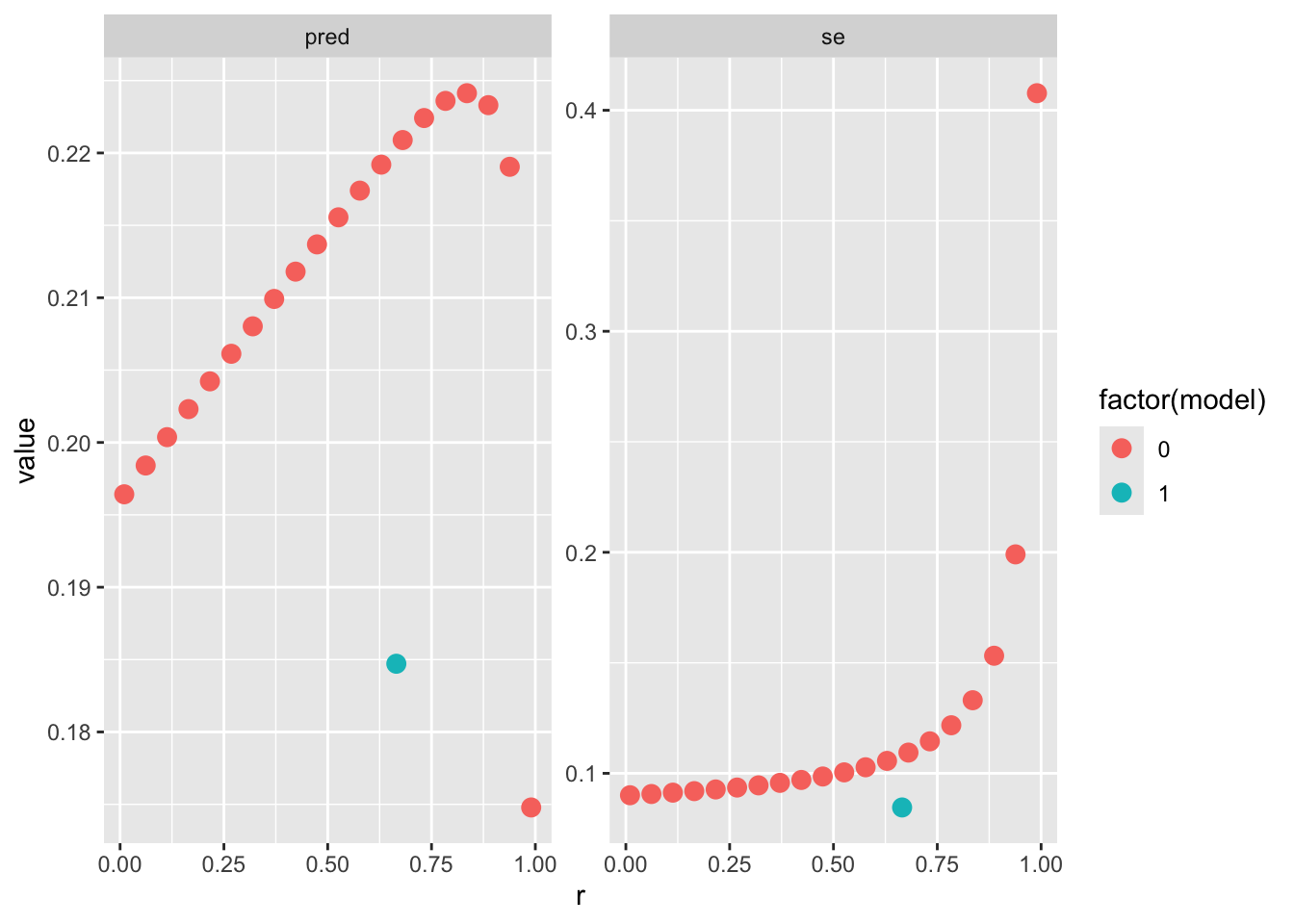
Checking the impact of using a different correlation compared to ICC:

r <- seq(0.01, 0.99, length.out = 20)
res <- vector(mode = "list", length = length(r))

for(i in 1:length(r)){
    V <- vcalc(vi, cluster = district, obs = study, rho = r[i], data = dat3l)
    fit <- rma.mv(yi, V, random = ~1|district, data = dat3l)
    fits <- data.frame(predict(fit))
    fits$sigma2 <- sum(fit$sigma2)
    fits$r <- r[i]
    res[[i]] <- fits
}

resd <- do.call(rbind, res)
resd$model <- 0

resd3l <- data.frame(predict(fit3l))
resd3l$sigma2 <- sum(fit3l.icc$tau2)
resd3l$r <- fit3l.icc$rho
resd3l$model <- 1

resd <- rbind(resd, resd3l)

resd |> 
    pivot_longer(c(pred, se)) |> 
    ggplot(aes(x = r, y = value, color = factor(model))) +
    geom_point(size = 3) +
    facet_wrap(~name, scales = "free")

Clearly, the assumption of the three-level model is that \(\omega^2\) is the same for each cluster thus we are estimating a single \(\omega^2\).

Simulating data

Data simulation again here is very useful to understand the model. We need to generate two vectors of random effects compared to the two-level model. Let’s start with a simple data structure with \(k\) clusters (e.g., papers) each having \(j\) nested effects.

k <- 30
j <- 3

dat <- expand.grid(
    effect = 1:j,
    paper = 1:k
)
dat$id <- 1:nrow(dat)
head(dat)
  effect paper id
1      1     1  1
2      2     1  2
3      3     1  3
4      1     2  4
5      2     2  5
6      3     2  6

Now we need to set the true parameters:

es <- 0.3
tau2 <- 0.15
omega2 <- 0.05
(icc <- tau2 / (tau2 + omega2)) # real icc
[1] 0.75
deltai <- rnorm(k, 0, tau2) # k random effects
zetaij <- rnorm(nrow(dat), 0, omega2) # k * j (or the number of rows) random effects

dat$deltai <- deltai[dat$paper]
dat$zetaij <- zetaij

# true effects
dat$thetai <- with(dat, es + deltai + zetaij)

head(dat)
  effect paper id      deltai       zetaij    thetai
1      1     1  1  0.10467002  0.020452242 0.4251223
2      2     1  2  0.10467002 -0.026584974 0.3780850
3      3     1  3  0.10467002 -0.006521141 0.3981489
4      1     2  4 -0.09007871 -0.055364805 0.1545565
5      2     2  5 -0.09007871 -0.052189956 0.1577313
6      3     2  6 -0.09007871 -0.009444707 0.2004766
dat |> 
    filter(paper %in% sample(unique(paper), 10)) |> 
    ggplot(aes(x = thetai, y = paper)) +
    geom_point(aes(color = factor(paper)))

Now we can use the usual sim_studies() function or manually to generate a study for each row of this dataframe with the true parameters.

dat$yi <- NA
dat$vi <- NA
dat$n0 <- 10 + rpois(nrow(dat), 50)
dat$n1 <- 10 + rpois(nrow(dat), 50)

for(i in 1:nrow(dat)){
    g0 <- rnorm(dat$n0[i], 0, 1)
    g1 <- rnorm(dat$n1[i], dat$thetai[i], 1)
    dat$yi[i] <- mean(g1) - mean(g0)
    dat$vi[i] <- var(g0)/dat$n0[i] + var(g1)/dat$n1[i]
}

fit <- rma.mv(yi, vi, random = ~ 1|paper/id, data = dat, sparse = TRUE)
fit.icc <- rma.mv(yi, vi, random = ~ effect|paper, data = dat, sparse = TRUE)

summary(fit)

Multivariate Meta-Analysis Model (k = 90; method: REML)

  logLik  Deviance       AIC       BIC      AICc   
  9.9399  -19.8798  -13.8798   -6.4138  -13.5974   

Variance Components:

            estim    sqrt  nlvls  fixed    factor 
sigma^2.1  0.0113  0.1063     30     no     paper 
sigma^2.2  0.0060  0.0778     90     no  paper/id 

Test for Heterogeneity:
Q(df = 89) = 133.1547, p-val = 0.0017

Model Results:

estimate      se    zval    pval   ci.lb   ci.ub      
  0.2734  0.0285  9.6072  <.0001  0.2176  0.3291  *** 

---
Signif. codes:  0 '***' 0.001 '**' 0.01 '*' 0.05 '.' 0.1 ' ' 1
summary(fit.icc)

Multivariate Meta-Analysis Model (k = 90; method: REML)

  logLik  Deviance       AIC       BIC      AICc   
  9.9399  -19.8798  -13.8798   -6.4138  -13.5974   

Variance Components:

outer factor: paper  (nlvls = 30)
inner factor: effect (nlvls = 3)

            estim    sqrt  fixed 
tau^2      0.0174  0.1317     no 
rho        0.6514             no 

Test for Heterogeneity:
Q(df = 89) = 133.1547, p-val = 0.0017

Model Results:

estimate      se    zval    pval   ci.lb   ci.ub      
  0.2734  0.0285  9.6072  <.0001  0.2176  0.3291  *** 

---
Signif. codes:  0 '***' 0.001 '**' 0.01 '*' 0.05 '.' 0.1 ' ' 1

We can put everything within a function to generate data also with heterogeneous number of effects \(j\) within each cluster.

sim_3l_studies <- function(k,
                           j,
                           es = 0,
                           tau2_k = 0,
                           tau2_j = 0,
                           n0,
                           n1 = NULL,
                           sample_j = FALSE,
                           sample_n = NULL,
                           simulate = TRUE,
                           raw = FALSE){
    if(sample_j){
        nj <- sample(1:j, k, replace = TRUE)
    } else{
        nj <- rep(j, k)
    }
    
    study <- unlist(lapply(nj, function(x) 1:x))
    paper <- rep(1:k, nj)
    sim <- data.frame(paper, study)
    
    delta_k <- rnorm(k, 0, sqrt(tau2_k))
    delta_j <- rnorm(nrow(sim), 0, sqrt(tau2_j))
    
    kj <- nrow(sim)
    
    if(!is.null(sample_n)){
        n0 <- round(sample_n(kj))
        n1 <- round(sample_n(kj))
    } else{
        if(length(n0) == 1) n0 <- rep(n0, nrow(sim))
        if(length(n1) == 1) n1 <- n0
    }
    
    es_kj <- es + delta_k[paper] + delta_j
    
    if(simulate){
        ss <- sim_studies(nrow(sim), es_kj, n0, n1, raw = raw)
        if(!raw){
            ss <- do.call(rbind, ss)
            res <- cbind(sim, ss)
        } else{
            res <- do.call(rbind, ss)
            paper_r <- rep(paper, sapply(ss, nrow))
            study_r <- rep(study, sapply(ss, nrow))
            res <- cbind(res, paper = paper_r, study = study_r)
        }
        
    } else{
        res <- sim
        res$es <- es
        res$delta_k <- delta_k[paper]
        res$delta_j <- delta_j
        res$theta_kj <- es_kj
    }
    
    return(res)
    
}

sim_study <- function(es, n0, n1, raw = FALSE){
    g0 <- rnorm(n0, 0, 1)
    g1 <- rnorm(n1, es, 1)
    
    if(raw){
        N <- n0 + n1
        out <- data.frame(
            subject = 1:N,
            x = rep(0:1, c(n0, n1)),
            y = c(g0, g1)
        )
    } else{
        yi <- mean(g1) - mean(g0)
        vi <- var(g0)/n0 + var(g1)/n1
        out <- data.frame(
            yi, vi
        )
    }
    return(out)
}

sim_studies <- function(k, es, n0, n1 = NULL, raw = FALSE){
    if(length(n0) == 1) n0 <- rep(n0, k)
    if(length(n1) == 1) n1 <- rep(n1, k) 
    if(is.null(n1)) n1 <- n0
    if(length(es) == 1) es <- rep(es, k)
    
    mapply(sim_study, es, n0, n1, raw = raw, SIMPLIFY = FALSE)
}

dat <- sim_3l_studies(k = 100, 
                      j = 5, 
                      es = 0.3, 
                      tau2_k = 0.1, 
                      tau2_j = 0.05, 
                      n0 = 50, 
                      n1 = 50)

fit.3l.sim <- rma.mv(yi, vi, random = ~ 1|paper/study, data = dat)
summary(fit.3l.sim)

Multivariate Meta-Analysis Model (k = 500; method: REML)

   logLik   Deviance        AIC        BIC       AICc   
-182.6122   365.2244   371.2244   383.8622   371.2729   

Variance Components:

            estim    sqrt  nlvls  fixed       factor 
sigma^2.1  0.1180  0.3435    100     no        paper 
sigma^2.2  0.0397  0.1992    500     no  paper/study 

Test for Heterogeneity:
Q(df = 499) = 2490.9682, p-val < .0001

Model Results:

estimate      se    zval    pval   ci.lb   ci.ub      
  0.2429  0.0366  6.6389  <.0001  0.1712  0.3146  *** 

---
Signif. codes:  0 '***' 0.001 '**' 0.01 '*' 0.05 '.' 0.1 ' ' 1

Similarly we can fit the corresponding model having the raw data to see the parameters estimated:

dat <- sim_3l_studies(k = 100, 
                      j = 5, 
                      es = 0.3, 
                      tau2_k = 0.1, 
                      tau2_j = 0.05, 
                      n0 = 50, 
                      n1 = 50,
                      raw = TRUE)

get_es <- function(data){
    dd <- data |> 
        group_by(x) |> 
        summarise(m = mean(y),
                  sd = sd(y),
                  n = n()) |> 
        pivot_wider(names_from = x, values_from = c(m, sd, n))
    escalc("MD", m1i = m_1, m2i = m_0, sd1i = sd_1, sd2i = sd_0, n1i = n_1, n2i = n_0,
           data = dd)
}

dat_agg <- dat |> 
    group_by(paper, study) |> 
    nest() |> 
    mutate(es = map(data, get_es)) |> 
    unnest(es) |> 
    select(-data)

fit3l <- rma.mv(yi, vi, random = ~1|paper/study, data = dat_agg)
summary(fit3l)

Multivariate Meta-Analysis Model (k = 500; method: REML)

   logLik   Deviance        AIC        BIC       AICc   
-194.6568   389.3136   395.3136   407.9514   395.3621   

Variance Components:

            estim    sqrt  nlvls  fixed       factor 
sigma^2.1  0.1021  0.3196    100     no        paper 
sigma^2.2  0.0477  0.2184    500     no  paper/study 

Test for Heterogeneity:
Q(df = 499) = 2384.5016, p-val < .0001

Model Results:

estimate      se    zval    pval   ci.lb   ci.ub      
  0.3256  0.0346  9.4164  <.0001  0.2579  0.3934  *** 

---
Signif. codes:  0 '***' 0.001 '**' 0.01 '*' 0.05 '.' 0.1 ' ' 1
dat$x <- factor(dat$x)
contrasts(dat$x) <- contr.sum(2)/2

fit3l.lmer <- lmer_alt(y ~ x + (x||paper/study), data = dat)
summary(fit3l.lmer)
Linear mixed model fit by REML. t-tests use Satterthwaite's method [
lmerModLmerTest]
Formula: y ~ x + (1 + re1.x1 || paper/study)
   Data: data

REML criterion at convergence: 143032.5

Scaled residuals: 
    Min      1Q  Median      3Q     Max 
-4.0132 -0.6696 -0.0016  0.6675  3.9603 

Random effects:
 Groups        Name        Variance Std.Dev.
 study.paper   re1.x1      0.04704  0.2169  
 study.paper.1 (Intercept) 0.01370  0.1171  
 paper         re1.x1      0.10271  0.3205  
 paper.1       (Intercept) 0.02670  0.1634  
 Residual                  0.99852  0.9993  
Number of obs: 50000, groups:  study:paper, 500; paper, 100

Fixed effects:
            Estimate Std. Error       df t value Pr(>|t|)    
(Intercept)  0.15610    0.01773 99.00121   8.803 4.43e-14 ***
x1          -0.32488    0.03466 98.99474  -9.374 2.54e-15 ***
---
Signif. codes:  0 '***' 0.001 '**' 0.01 '*' 0.05 '.' 0.1 ' ' 1

Correlation of Fixed Effects:
   (Intr)
x1 0.000 

Multivariate meta-analysis

As introduced at the beginning the term multivariate is used here for data structure where the dependency arises from multiple effects being collected on the same pool of participants.

For example, in each primary study we did a group comparison (between two independent groups) on two measures. The two effect sizes are correlated because they are measured on the same participants.

The data structure is essentially the same but sampling errors are now correlated within clusters.

dat.mv <- expand.grid(
    outcome = 1:2,
    paper = 1:10
)

head(dat.mv)
  outcome paper
1       1     1
2       2     1
3       1     2
4       2     2
5       1     3
6       2     3

How a single study looks like?

n0 <- 50
n1 <- 50

d <- c(0.3, 0.5)

r <- 0.6
R <- r + diag(1 - r, 2)

g0 <- MASS::mvrnorm(n0, c(0, 0), R)
g1 <- MASS::mvrnorm(n0, d, R)

m0 <- apply(g0, 2, mean)
m1 <- apply(g1, 2, mean)

v0 <- apply(g0, 2, var)
v1 <- apply(g1, 2, var)

yi <- m1 - m0
vi <- v0/n0 + v1/n1
ri <- cor(rbind(g0, g1))
vvi <- diag(sqrt(vi)) %*% ri %*% diag(sqrt(vi))
vvi <- data.frame(vvi)
names(vvi) <- c("v1i", "v2i")

cbind(yi, vi, vvi, n0, n1, outcome = c(1, 2))
         yi         vi        v1i        v2i n0 n1 outcome
1 0.3330190 0.04401455 0.04401455 0.02350021 50 50       1
2 0.2875695 0.03896922 0.02350021 0.03896922 50 50       2

We have two effects, two sampling variances and their correlation/covariance.

Formally the model (for a single study) can be written as:

\[\begin{align} \begin{gathered} \begin{bmatrix} y_{1_i} \\ y_{2_i} \\ y_{3_i} \end{bmatrix} = \begin{bmatrix} \mu_{{\theta}_{1}} \\ \mu_{{\theta}_{2}} \\ \mu_{{\theta}_{3}} \end{bmatrix} + \begin{bmatrix} \delta_{1_i} \\ \delta_{2_i} \\ \delta_{3_i} \end{bmatrix} + \begin{bmatrix} \epsilon_{1_i} \\ \epsilon_{2_i} \\ \epsilon_{3_i} \end{bmatrix} \end{gathered} \end{align}\]

\[\begin{align} \begin{gathered} \begin{bmatrix} \delta_{1_i} \\ \delta_{2_i} \\ \delta_{3_i} \end{bmatrix} \sim \mathcal{MVN}(0, \mathrm{T}) \end{gathered} \end{align}\]

\[\begin{align} \begin{gathered} \begin{bmatrix} \epsilon_{1_i} \\ \epsilon_{2_i} \\ \epsilon_{3_i} \end{bmatrix} \sim \mathcal{MVN}(0, \mathrm{V}) \end{gathered} \end{align}\]

\[\begin{align} \begin{gathered} \mathrm{T} = \begin{bmatrix} \tau_1^2 & & & \\ \rho_{21}\tau_2\tau_1 & \tau_2^2 & & \\ \rho_{31}\tau_3\tau_1 & \rho_{32}\tau_3\tau_2 & \tau_3^2 \end{bmatrix} \end{gathered} \end{align}\]

\[\begin{align} \begin{gathered} \mathrm{V} = \begin{bmatrix} \sigma^2_{\epsilon_1} & & & \\ \rho_{s_{21}}\sigma_{\epsilon_2}\sigma_{\epsilon_1} & \sigma^2_{\epsilon_2} & & \\ \rho_{s_{31}}\sigma_{\epsilon_3}\sigma_{\epsilon_1} & \rho_{s_{32}}\sigma_{\epsilon_3}\sigma_{\epsilon_2} & \sigma^2_{\epsilon_3} \end{bmatrix} \end{gathered} \end{align}\]

The \(\mbox{V}\) matrix is the same that we created with vcalc. Basically is a block variance-covariance matrix with \(k\) matrices (one for each paper/cluster) and number of rows/columns depending on how many outcomes are collected for each paper.

The \(\mbox{T}\) is a \(p\times p\) matrix with \(p\) being the number of outcomes that represents the random-effects matrix. The diagonal is the true heterogeneity across studies for each outcome and the off-diagonal elements are the correlations between different outcomes across studies.

The multivariate model needs \(\mbox{V}\) (as the vi vector) and estimates \(\mbox{T}\) along with the vector of effect sizes.

Let’s see an example with the dat.berkey1998 dataset (see also https://www.metafor-project.org/doku.php/analyses:berkey1998)

dat <- dat.berkey1998
dat

   trial           author year ni outcome      yi     vi    v1i    v2i 
1      1 Pihlstrom et al. 1983 14      PD  0.4700 0.0075 0.0075 0.0030 
2      1 Pihlstrom et al. 1983 14      AL -0.3200 0.0077 0.0030 0.0077 
3      2    Lindhe et al. 1982 15      PD  0.2000 0.0057 0.0057 0.0009 
4      2    Lindhe et al. 1982 15      AL -0.6000 0.0008 0.0009 0.0008 
5      3   Knowles et al. 1979 78      PD  0.4000 0.0021 0.0021 0.0007 
6      3   Knowles et al. 1979 78      AL -0.1200 0.0014 0.0007 0.0014 
7      4  Ramfjord et al. 1987 89      PD  0.2600 0.0029 0.0029 0.0009 
8      4  Ramfjord et al. 1987 89      AL -0.3100 0.0015 0.0009 0.0015 
9      5    Becker et al. 1988 16      PD  0.5600 0.0148 0.0148 0.0072 
10     5    Becker et al. 1988 16      AL -0.3900 0.0304 0.0072 0.0304 

Berkey et al. (1998) describe a meta-analytic multivariate model for the analysis of multiple correlated outcomes. The use of the model is illustrated with results from 5 trials comparing surgical and non-surgical treatments for medium-severity periodontal disease. Reported outcomes include the change in probing depth (PD) and attachment level (AL) one year after the treatment. The effect size measure used for this meta-analysis was the (raw) mean difference, calculated in such a way that positive values indicate that surgery was more effective than non-surgical treatment in decreasing the probing depth and increasing the attachment level.

We need to create the V matrix:

V <- vcalc(vi=1, cluster=author, rvars=c(v1i, v2i), data=dat)
round(V, 3)
       [,1]  [,2]  [,3]  [,4]  [,5]  [,6]  [,7]  [,8]  [,9] [,10]
 [1,] 0.007 0.003 0.000 0.000 0.000 0.000 0.000 0.000 0.000 0.000
 [2,] 0.003 0.008 0.000 0.000 0.000 0.000 0.000 0.000 0.000 0.000
 [3,] 0.000 0.000 0.006 0.001 0.000 0.000 0.000 0.000 0.000 0.000
 [4,] 0.000 0.000 0.001 0.001 0.000 0.000 0.000 0.000 0.000 0.000
 [5,] 0.000 0.000 0.000 0.000 0.002 0.001 0.000 0.000 0.000 0.000
 [6,] 0.000 0.000 0.000 0.000 0.001 0.001 0.000 0.000 0.000 0.000
 [7,] 0.000 0.000 0.000 0.000 0.000 0.000 0.003 0.001 0.000 0.000
 [8,] 0.000 0.000 0.000 0.000 0.000 0.000 0.001 0.002 0.000 0.000
 [9,] 0.000 0.000 0.000 0.000 0.000 0.000 0.000 0.000 0.015 0.007
[10,] 0.000 0.000 0.000 0.000 0.000 0.000 0.000 0.000 0.007 0.030
blsplit(V, dat$author, fun = round, 3)
$`Pihlstrom et al.`
      [,1]  [,2]
[1,] 0.007 0.003
[2,] 0.003 0.008

$`Lindhe et al.`
      [,1]  [,2]
[1,] 0.006 0.001
[2,] 0.001 0.001

$`Knowles et al.`
      [,1]  [,2]
[1,] 0.002 0.001
[2,] 0.001 0.001

$`Ramfjord et al.`
      [,1]  [,2]
[1,] 0.003 0.001
[2,] 0.001 0.002

$`Becker et al.`
      [,1]  [,2]
[1,] 0.015 0.007
[2,] 0.007 0.030

Then the model is the same as the three-level model with the ICC parametrization:

fit.mv0 <- rma.mv(yi, V, random = ~outcome|trial, data = dat, struct = "UN")
fit.mv0

Multivariate Meta-Analysis Model (k = 10; method: REML)

Variance Components:

outer factor: trial   (nlvls = 5)
inner factor: outcome (nlvls = 2)

            estim    sqrt  k.lvl  fixed  level 
tau^2.1    0.3571  0.5976      5     no     AL 
tau^2.2    0.0356  0.1887      5     no     PD 

     rho.AL  rho.PD    AL  PD 
AL        1             -   5 
PD  -0.6678       1    no   - 

Test for Heterogeneity:
Q(df = 9) = 784.6078, p-val < .0001

Model Results:

estimate      se    zval    pval   ci.lb   ci.ub      
  0.2154  0.0592  3.6369  0.0003  0.0993  0.3315  *** 

---
Signif. codes:  0 '***' 0.001 '**' 0.01 '*' 0.05 '.' 0.1 ' ' 1

What is missing is the fixed part. We are estimating an average outcome effect because we are not differentiating between outcomes. We just need to include outcome as a moderator:

fit.mv1 <- rma.mv(yi, V, 
                  mods = ~ 0 + outcome, 
                  random = ~ outcome|trial, 
                  data = dat, struct = "UN")
fit.mv1

Multivariate Meta-Analysis Model (k = 10; method: REML)

Variance Components:

outer factor: trial   (nlvls = 5)
inner factor: outcome (nlvls = 2)

            estim    sqrt  k.lvl  fixed  level 
tau^2.1    0.0327  0.1807      5     no     AL 
tau^2.2    0.0117  0.1083      5     no     PD 

    rho.AL  rho.PD    AL  PD 
AL       1             -   5 
PD  0.6088       1    no   - 

Test for Residual Heterogeneity:
QE(df = 8) = 128.2267, p-val < .0001

Test of Moderators (coefficients 1:2):
QM(df = 2) = 108.8616, p-val < .0001

Model Results:

           estimate      se     zval    pval    ci.lb    ci.ub      
outcomeAL   -0.3392  0.0879  -3.8589  0.0001  -0.5115  -0.1669  *** 
outcomePD    0.3534  0.0588   6.0057  <.0001   0.2381   0.4688  *** 

---
Signif. codes:  0 '***' 0.001 '**' 0.01 '*' 0.05 '.' 0.1 ' ' 1

Now we have the estimated treatment effect and the \(\mbox{T}\) matrix.

Multivariate as three-level model

Sometimes, the correlations between outcomes are missing and we need to put a plausible value. Van den Noortgate et al. (2013) showed that under some assumptions, fitting a three-level model (thus assuming independence) is actually estimating the effects and standard error in a similar way as the multivariate model including or guessing a correlation.

fit.mv1 <- rma.mv(yi, V, 
                  mods = ~ 0 + outcome, 
                  random = ~ outcome|trial, 
                  data = dat, 
                  struct = "CS")

fit.mv.3l <- rma.mv(yi, 
                    vi, 
                    mods = ~ 0 + outcome, 
                    random = ~ 1|trial/outcome, 
                    data = dat)


fit.mv1

Multivariate Meta-Analysis Model (k = 10; method: REML)

Variance Components:

outer factor: trial   (nlvls = 5)
inner factor: outcome (nlvls = 2)

            estim    sqrt  fixed 
tau^2      0.0250  0.1582     no 
rho        0.5290             no 

Test for Residual Heterogeneity:
QE(df = 8) = 128.2267, p-val < .0001

Test of Moderators (coefficients 1:2):
QM(df = 2) = 79.9819, p-val < .0001

Model Results:

           estimate      se     zval    pval    ci.lb    ci.ub      
outcomeAL   -0.3380  0.0782  -4.3229  <.0001  -0.4912  -0.1847  *** 
outcomePD    0.3636  0.0788   4.6163  <.0001   0.2092   0.5180  *** 

---
Signif. codes:  0 '***' 0.001 '**' 0.01 '*' 0.05 '.' 0.1 ' ' 1
fit.mv.3l

Multivariate Meta-Analysis Model (k = 10; method: REML)

Variance Components:

            estim    sqrt  nlvls  fixed         factor 
sigma^2.1  0.0143  0.1196      5     no          trial 
sigma^2.2  0.0102  0.1012     10     no  trial/outcome 

Test for Residual Heterogeneity:
QE(df = 8) = 124.9021, p-val < .0001

Test of Moderators (coefficients 1:2):
QM(df = 2) = 78.0792, p-val < .0001

Model Results:

           estimate      se     zval    pval    ci.lb    ci.ub      
outcomeAL   -0.3323  0.0772  -4.3041  <.0001  -0.4836  -0.1810  *** 
outcomePD    0.3594  0.0780   4.6056  <.0001   0.2064   0.5123  *** 

---
Signif. codes:  0 '***' 0.001 '**' 0.01 '*' 0.05 '.' 0.1 ' ' 1

The advantage is that in the three-level model we are not imputing values.

Simulating data

sim_multi_meta <- function(k, 
                           p,
                           mus,
                           tau2s,
                           ro = 0,
                           rs = 0,
                           n = NULL,
                           sample_p = FALSE,
                           sample_n = NULL,
                           ranef = FALSE){
    
    RT <- ro + diag(1 - ro, p)
    RS <- rs + diag(1 - rs, p)
    S <- diag(sqrt(tau2s)) %*% RT %*% diag(sqrt(tau2s))
    
    TT <- MASS::mvrnorm(k, rep(0, p), S)
    
    yi <- vi <- deltai <- vvi <- vector(mode = "list", length = k)
    
    for(i in 1:k){
        X0 <- MASS::mvrnorm(n, rep(0, p), RS)
        X1 <- MASS::mvrnorm(n, mus + TT[i, ], RS)
        mm0 <- apply(X0, 2, mean)
        mm1 <- apply(X1, 2, mean)
        
        vv01 <- cov(X0)/n + cov(X1)/n
        
        yi[[i]] <- mm1 - mm0
        vi[[i]] <- diag(vv01)
        
        vvi[[i]] <- vv01
        deltai[[i]] <- TT[i, ]
    }
    
    if(sample_p){
        pi <- sample(1:p, k, replace = TRUE)
    } else{
        pi <- rep(p, k)
    }
    
    study <- rep(1:k, each = p)
    outcome <- rep(1:p, k)
    
    sim <- data.frame(
        study,
        outcome
    )
    
    sim$yi <- unlist(yi)
    sim$vi <- unlist(vi)
    
    vvi <- do.call(rbind, vvi)
    vvi <- data.frame(vvi)
    names(vvi) <- sprintf("v%si", 1:ncol(vvi))
    
    sim <- cbind(sim, vvi)
    
    if(ranef){
        sim$deltai <- unlist(deltai)
    }
    
    # selecting studies
    siml <- split(sim, sim$study)
    for(i in 1:k){
        siml[[i]] <- siml[[i]][1:pi[i], ]
    }
    sim <- do.call(rbind, siml)
    sim$outcome <- factor(paste0("o", sim$outcome))
    rownames(sim) <- NULL
    return(sim)
}

dat <- sim_multi_meta(k = 10, 
               p = 3, 
               mus = c(0, 0, 0), 
               tau2s = c(0.1, 0.1, 0.1), 
               ro = 0.5, 
               rs = 0.5, 
               n = 100)

V <- vcalc(vi = 1, cluster = study, rvars = c(v1i, v2i, v3i), data = dat)

fit.mv <- rma.mv(yi, 
                 V, 
                 mods = ~ 0 + outcome, 
                 random = ~ outcome|study, 
                 data = dat)

fit.mv

Multivariate Meta-Analysis Model (k = 30; method: REML)

Variance Components:

outer factor: study   (nlvls = 10)
inner factor: outcome (nlvls = 3)

            estim    sqrt  fixed 
tau^2      0.1425  0.3775     no 
rho        0.7375             no 

Test for Residual Heterogeneity:
QE(df = 27) = 174.7938, p-val < .0001

Test of Moderators (coefficients 1:3):
QM(df = 3) = 5.2444, p-val = 0.1548

Model Results:

           estimate      se     zval    pval    ci.lb   ci.ub    
outcomeo1    0.1345  0.1274   1.0554  0.2912  -0.1152  0.3841    
outcomeo2   -0.0430  0.1272  -0.3381  0.7353  -0.2922  0.2062    
outcomeo3    0.1455  0.1271   1.1445  0.2524  -0.1037  0.3947    

---
Signif. codes:  0 '***' 0.001 '**' 0.01 '*' 0.05 '.' 0.1 ' ' 1
fit.mv.3l <- rma.mv(yi, 
                 vi, 
                 mods = ~ 0 + outcome, 
                 random = ~ 1|outcome/study, 
                 data = dat)

fit.mv.3l

Multivariate Meta-Analysis Model (k = 30; method: REML)

Variance Components:

            estim    sqrt  nlvls  fixed         factor 
sigma^2.1  0.0333  0.1825      3     no        outcome 
sigma^2.2  0.1424  0.3774     30     no  outcome/study 

Test for Residual Heterogeneity:
QE(df = 27) = 219.2477, p-val < .0001

Test of Moderators (coefficients 1:3):
QM(df = 3) = 0.8082, p-val = 0.8475

Model Results:

           estimate      se     zval    pval    ci.lb   ci.ub    
outcomeo1    0.1341  0.2226   0.6025  0.5468  -0.3021  0.5704    
outcomeo2   -0.0406  0.2225  -0.1826  0.8551  -0.4766  0.3954    
outcomeo3    0.1427  0.2224   0.6418  0.5210  -0.2932  0.5787    

---
Signif. codes:  0 '***' 0.001 '**' 0.01 '*' 0.05 '.' 0.1 ' ' 1

References

Van den Noortgate, Wim, José Antonio López-López, Fulgencio Marín-Martínez, and Julio Sánchez-Meca. 2013. “Three-Level Meta-Analysis of Dependent Effect Sizes.” Behavior Research Methods 45 (June): 576–94. https://doi.org/10.3758/s13428-012-0261-6.