Useful GLMER tools

Author

Filippo Gambarota

Equations from models

library(lme4)
library(equatiomatic)

fit_lme4 <- lmer(Reaction ~ Days + (Days|Subject), data = sleepstudy)
equatiomatic::extract_eq(fit_lme4)

\[ \begin{aligned} \operatorname{Reaction}_{i} &\sim N \left(\alpha_{j[i]} + \beta_{1j[i]}(\operatorname{Days}), \sigma^2 \right) \\ \left( \begin{array}{c} \begin{aligned} &\alpha_{j} \\ &\beta_{1j} \end{aligned} \end{array} \right) &\sim N \left( \left( \begin{array}{c} \begin{aligned} &\mu_{\alpha_{j}} \\ &\mu_{\beta_{1j}} \end{aligned} \end{array} \right) , \left( \begin{array}{cc} \sigma^2_{\alpha_{j}} & \rho_{\alpha_{j}\beta_{1j}} \\ \rho_{\beta_{1j}\alpha_{j}} & \sigma^2_{\beta_{1j}} \end{array} \right) \right) \text{, for Subject j = 1,} \dots \text{,J} \end{aligned} \]

Plotting effects

library(effects)
plot(allEffects(fit_lme4))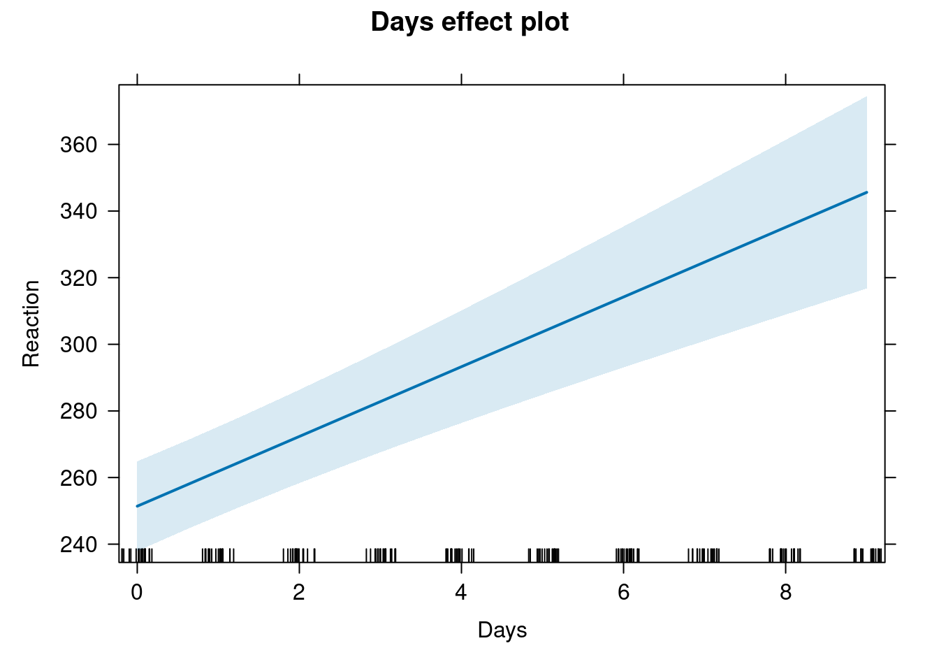

library(ggeffects)
library(ggplot2)

plot(ggeffect(fit_lme4)) +
    ggtitle("Amazing Title")

Marginal effects

library(emmeans)

fit <- lm(Sepal.Length ~ Petal.Width * Species, data = iris)
emmeans(fit, ~ Species)

 Species    emmean     SE  df lower.CL upper.CL
 setosa       5.89 0.6225 144     4.66     7.12
 versicolor   5.76 0.0807 144     5.60     5.91
 virginica    6.05 0.2168 144     5.62     6.48

Confidence level used: 0.95

# comparisons
emmeans(fit, pairwise ~ Species)

$emmeans
 Species    emmean     SE  df lower.CL upper.CL
 setosa       5.89 0.6225 144     4.66     7.12
 versicolor   5.76 0.0807 144     5.60     5.91
 virginica    6.05 0.2168 144     5.62     6.48

Confidence level used: 0.95 

$contrasts
 contrast               estimate    SE  df t.ratio p.value
 setosa - versicolor       0.137 0.628 144   0.219  0.9739
 setosa - virginica       -0.157 0.659 144  -0.238  0.9691
 versicolor - virginica   -0.295 0.231 144  -1.274  0.4121

P value adjustment: tukey method for comparing a family of 3 estimates

# comparison fixing Petal.Width
emmeans(fit, pairwise ~ Species, at = list(Petal.Width = 1))

$emmeans
 Species    emmean    SE  df lower.CL upper.CL
 setosa       5.71 0.494 144     4.73     6.68
 versicolor   5.47 0.132 144     5.21     5.73
 virginica    5.92 0.264 144     5.40     6.44

Confidence level used: 0.95 

$contrasts
 contrast               estimate    SE  df t.ratio p.value
 setosa - versicolor       0.236 0.511 144   0.462  0.8890
 setosa - virginica       -0.213 0.560 144  -0.380  0.9236
 versicolor - virginica   -0.449 0.295 144  -1.521  0.2840

P value adjustment: tukey method for comparing a family of 3 estimates

# comparison of slopes

emtrends(fit, ~ Species, var = "Petal.Width")

 Species    Petal.Width.trend    SE  df lower.CL upper.CL
 setosa                 0.930 0.649 144   -0.353     2.21
 versicolor             1.426 0.346 144    0.743     2.11
 virginica              0.651 0.249 144    0.159     1.14

Confidence level used: 0.95

emtrends(fit, pairwise ~ Species, var = "Petal.Width")

$emtrends
 Species    Petal.Width.trend    SE  df lower.CL upper.CL
 setosa                 0.930 0.649 144   -0.353     2.21
 versicolor             1.426 0.346 144    0.743     2.11
 virginica              0.651 0.249 144    0.159     1.14

Confidence level used: 0.95 

$contrasts
 contrast               estimate    SE  df t.ratio p.value
 setosa - versicolor      -0.496 0.736 144  -0.675  0.7786
 setosa - virginica        0.279 0.695 144   0.402  0.9149
 versicolor - virginica    0.776 0.426 144   1.819  0.1669

P value adjustment: tukey method for comparing a family of 3 estimates

# factorial designs
warp.lm <- lm(breaks ~ wool * tension, data = warpbreaks)
emmeans (warp.lm,  pairwise ~ wool | tension)

$emmeans
tension = L:
 wool emmean   SE df lower.CL upper.CL
 A      44.6 3.65 48     37.2     51.9
 B      28.2 3.65 48     20.9     35.6

tension = M:
 wool emmean   SE df lower.CL upper.CL
 A      24.0 3.65 48     16.7     31.3
 B      28.8 3.65 48     21.4     36.1

tension = H:
 wool emmean   SE df lower.CL upper.CL
 A      24.6 3.65 48     17.2     31.9
 B      18.8 3.65 48     11.4     26.1

Confidence level used: 0.95 

$contrasts
tension = L:
 contrast estimate   SE df t.ratio p.value
 A - B       16.33 5.16 48   3.167  0.0027

tension = M:
 contrast estimate   SE df t.ratio p.value
 A - B       -4.78 5.16 48  -0.926  0.3589

tension = H:
 contrast estimate   SE df t.ratio p.value
 A - B        5.78 5.16 48   1.120  0.2682

Also the marginaleffects package is amazing.

Tables

library(sjPlot)

tab_model(fit)

	Sepal.Length
Predictors	Estimates	CI	p
(Intercept)	4.78	4.43 – 5.12	<0.001
Petal Width	0.93	-0.35 – 2.21	0.154
Species [versicolor]	-0.73	-1.71 – 0.25	0.141
Species [virginica]	0.49	-0.57 – 1.56	0.362
Petal Width × Species [versicolor]	0.50	-0.96 – 1.95	0.501
Petal Width × Species [virginica]	-0.28	-1.65 – 1.09	0.688
Observations	150
R² / R² adjusted	0.677 / 0.666

tab_model(fit_lme4)

	Reaction
Predictors	Estimates	CI	p
(Intercept)	251.41	237.94 – 264.87	<0.001
Days	10.47	7.42 – 13.52	<0.001
Random Effects
σ²	654.94
τ₀₀ _Subject	612.10
τ₁₁ _Subject.Days	35.07
ρ₀₁ _Subject	0.07
ICC	0.72
N _Subject	18
Observations	180
Marginal R² / Conditional R²	0.279 / 0.799

library(gtsummary)

gtsummary::tbl_regression(fit_lme4)

Characteristic	Beta	95% CI
Days	10	7.4, 13
Abbreviation: CI = Confidence Interval