2025-04-08

Simuliamo dati fissando una certa correlazione pre-post come ICC:

library(lme4)

n <- 1e4
r <- 0.7 # icc = r
b0 <- 0
b1 <- 0.3
sb0 <- sqrt(r)
s <- sqrt(1 - sb0^2)

dat <- data.frame(
    x = rep(0:1, each = n),
    id = rep(1:n, 2)
)

b0i <- rnorm(n, 0, sb0)
dat$y <- rnorm(n*2, with(dat, b0 + b0i[id] + b1 * x), s)

fit <- lmer(y ~ x + (1|id), data = dat)
summary(fit)

Linear mixed model fit by REML ['lmerMod']
Formula: y ~ x + (1 | id)
   Data: dat

REML criterion at convergence: 50018.8

Scaled residuals: 
    Min      1Q  Median      3Q     Max 
-3.1288 -0.5133 -0.0030  0.5213  3.2586 

Random effects:
 Groups   Name        Variance Std.Dev.
 id       (Intercept) 0.6961   0.8343  
 Residual             0.3007   0.5484  
Number of obs: 20000, groups:  id, 10000

Fixed effects:
             Estimate Std. Error t value
(Intercept) -0.008000   0.009984  -0.801
x            0.303728   0.007755  39.166

Correlation of Fixed Effects:
  (Intr)
x -0.388

sb0^2 / (sb0^2 + s^2)

[1] 0.7

summary(fit)

Linear mixed model fit by REML ['lmerMod']
Formula: y ~ x + (1 | id)
   Data: dat

REML criterion at convergence: 50018.8

Scaled residuals: 
    Min      1Q  Median      3Q     Max 
-3.1288 -0.5133 -0.0030  0.5213  3.2586 

Random effects:
 Groups   Name        Variance Std.Dev.
 id       (Intercept) 0.6961   0.8343  
 Residual             0.3007   0.5484  
Number of obs: 20000, groups:  id, 10000

Fixed effects:
             Estimate Std. Error t value
(Intercept) -0.008000   0.009984  -0.801
x            0.303728   0.007755  39.166

Correlation of Fixed Effects:
  (Intr)
x -0.388

performance::icc(fit)

# Intraclass Correlation Coefficient

    Adjusted ICC: 0.698
  Unadjusted ICC: 0.683

Simuliamo random-intercepts e slopes con anche l’effetto di una covariata al livello del soggetto.

n <- 10
nt <- 10

age <- round(runif(n, 20, 30))

dat <- expand.grid(
    id = 1:n,
    trial = 1:nt,
    x = c(0, 1)
)

dat$age <- age[dat$id]

b0 <- 0.1
b1 <- 0.5
b2 <- 0.1
sb0 <- 0.2
sb1 <- 0.1
s <- 1

rb0b1 <- 0.5

R <- rb0b1 + diag(1 - rb0b1, 2)
S <- diag(c(sb0, sb1)) %*% R %*% diag(c(sb0, sb1))

Z <- MASS::mvrnorm(n, c(0, 0), S)

b0i <- Z[, 1]
b1i <- Z[, 2]

dat$age0 <- dat$age - mean(dat$age)
dat$lp <- b0 + b0i[dat$id] + (b1 + b1i[dat$id]) * dat$x + b2 * dat$age0
dat$y <- rnorm(nrow(dat), dat$lp, s)
fit <- lmer(y ~ x + age + (x|id), dat = dat)

summary(fit)

Linear mixed model fit by REML ['lmerMod']
Formula: y ~ x + age + (x | id)
   Data: dat

REML criterion at convergence: 582.7

Scaled residuals: 
    Min      1Q  Median      3Q     Max 
-3.2763 -0.5854  0.0459  0.6215  2.4063 

Random effects:
 Groups   Name        Variance  Std.Dev. Corr
 id       (Intercept) 7.060e-02 0.265698     
          x           4.231e-06 0.002057 1.00
 Residual             9.979e-01 0.998936     
Number of obs: 200, groups:  id, 10

Fixed effects:
            Estimate Std. Error t value
(Intercept) -3.03737    0.87610  -3.467
x            0.35413    0.14127   2.507
age          0.12548    0.03282   3.824

Correlation of Fixed Effects:
    (Intr) x     
x   -0.080       
age -0.989  0.000
optimizer (nloptwrap) convergence code: 0 (OK)
boundary (singular) fit: see help('isSingular')

performance::r2(fit)

Random effect variances not available. Returned R2 does not account for random effects.

# R2 for Mixed Models

  Conditional R2: NA
     Marginal R2: 0.173

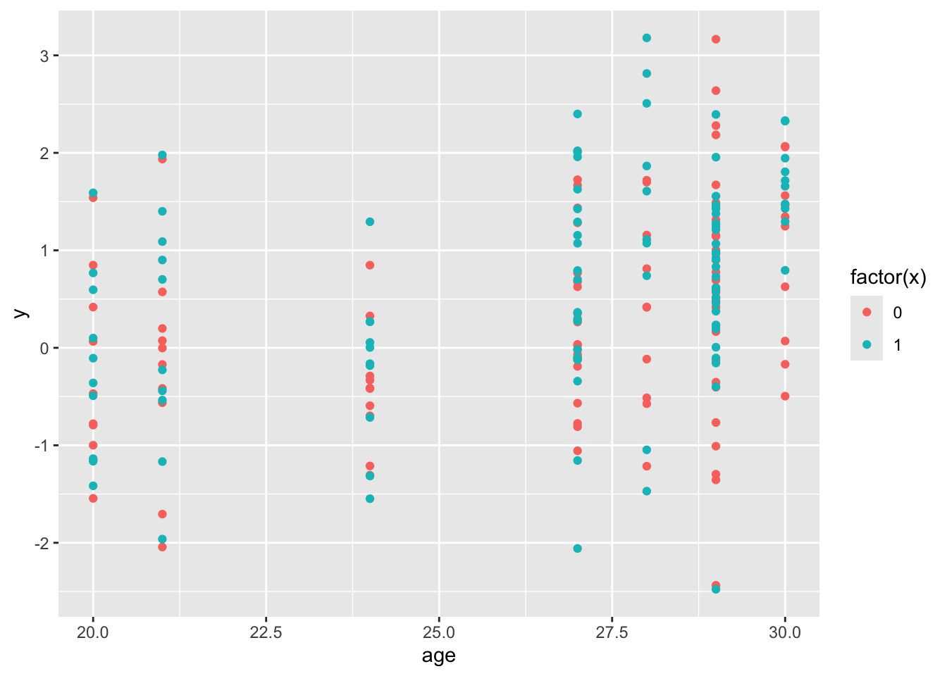
library(ggplot2)

dat |> 
    ggplot(aes(x = age, y = y)) +
    geom_point(aes(color = factor(x)))

Simuliamo un modello logit:

n <- 100
nt <- 1e3
b0 <- qlogis(0.01)
b1 <- 10
sb0 <- 1

# plogis(qlogis(0.01) + rnorm(1e4, 0, sb0)) |> 
#     hist()


dd <- expand.grid(
    id = 1:n,
    nt = 1:nt
)

dd$x <- runif(nrow(dd), 0, 1)
b0i <- rnorm(n, 0, sb0)

dd$lp <-  + b1 * dd$x
dd$p <- plogis(dd$lp)

# dd |> 
#     ggplot(aes(x = x, y = p, group = id)) +
#     geom_line()

dd$y <- rbinom(nrow(dd), 1, dd$p)

library(lme4)

fit <- glmer(y ~ x + (1|id),
             data = dd, 
             family = binomial())

performance::icc(fit)

[1] NA

summary(fit)

Generalized linear mixed model fit by maximum likelihood (Laplace
  Approximation) [glmerMod]
 Family: binomial  ( logit )
Formula: y ~ x + (1 | id)
   Data: dd

      AIC       BIC    logLik -2*log(L)  df.resid 
  32799.4   32828.0  -16396.7   32793.4     99997 

Scaled residuals: 
    Min      1Q  Median      3Q     Max 
-67.165   0.016   0.056   0.204   1.008 

Random effects:
 Groups Name        Variance Std.Dev.
 id     (Intercept) 0        0       
Number of obs: 100000, groups:  id, 100

Fixed effects:
            Estimate Std. Error z value Pr(>|z|)    
(Intercept) -0.01598    0.02193  -0.729    0.466    
x           10.12262    0.12273  82.476   <2e-16 ***
---
Signif. codes:  0 '***' 0.001 '**' 0.01 '*' 0.05 '.' 0.1 ' ' 1

Correlation of Fixed Effects:
  (Intr)
x -0.764
optimizer (Nelder_Mead) convergence code: 0 (OK)
boundary (singular) fit: see help('isSingular')

# intraclass correlation con varianza della logistica come costante
0.8821 / (0.8821 + pi^2/3)

[1] 0.211435