Modern R

Psicometria per le Neuroscienze Cognitive

Filippo Gambarota, PhD

Reproducibility starter pack

Reproducibility starter pack 👷

A general purpose (or flexible enough) programming language such as or
A literate programming framework to integrate code and text
A version control system to track projects
An online repository for future-proof sharing

Disclaimers

The best tool is the tool that does the job.

But there are some features that makes a tool better in terms of reproducibility, reducing the probability of errors and improve your coding skills.
There is nothing bad about using SPSS, Jasp or Jamovi. The real problem is that using a point-and-click software reduce the reproducibility. If you can use the scripting part, whatever the tool.
A general suggestion is to invest some of your time learning/improving a programming language for data pre-processing, analysis and reporting (tables, figures, etc.)

R Programming Language

R

R is a free software environment for statistical computing and graphics.

(TBH) It is not a proper general purpose programming language (such as C++ or Python).
R packages allow to do almost everything (file manager, image processing, webscraping, sending emails, coffee 😄, etc.)
It is free and open-source
The community is wide, active thus solving problems is very easy
Force you to learn scripting but the are R-based GUI software (e.g., JAMOVI)

R - CRAN

The CRAN is the repository where package developers upload their packages and other users can install them.

As the saying goes: if something exist, there is an R package for doing it! 😄

R - PYPL Index

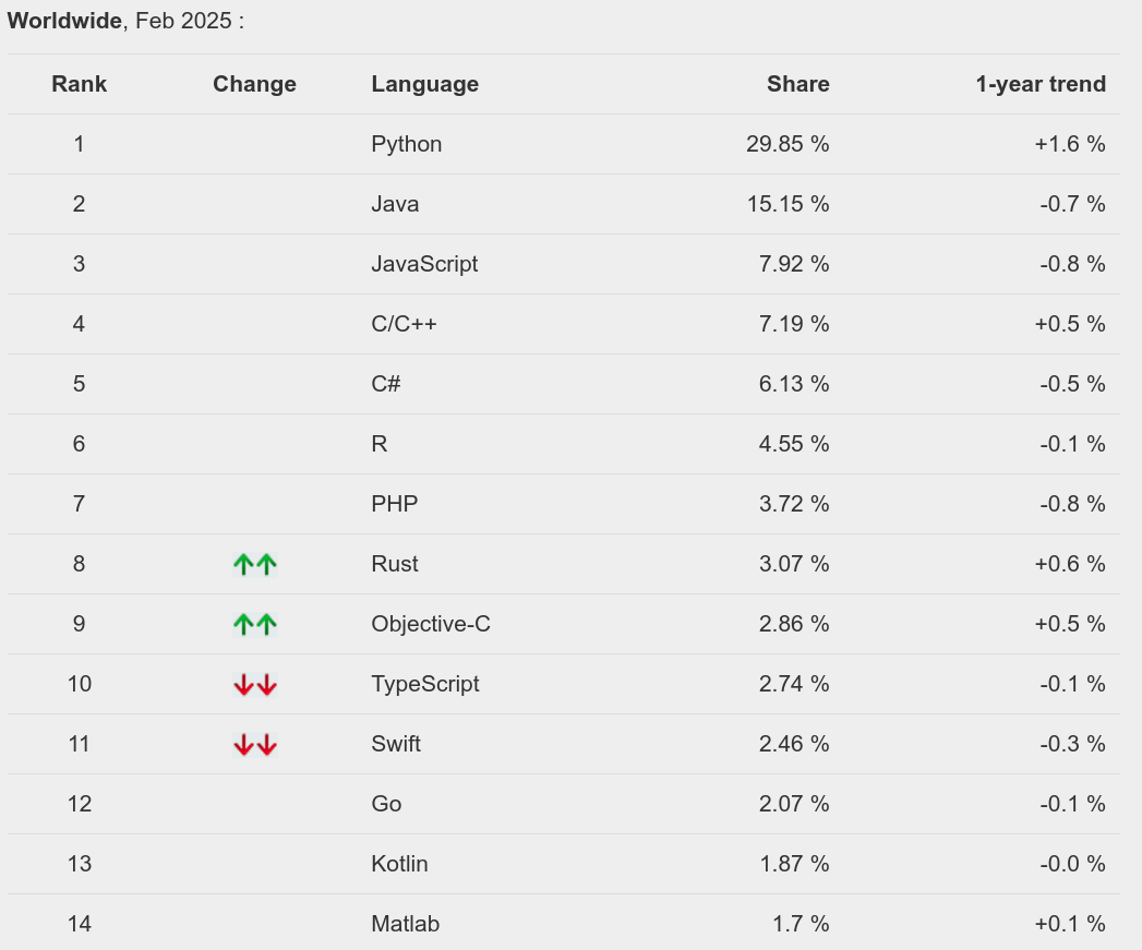
Source: https://pypl.github.io/PYPL.html

R - PYPL Index

The popularity is on a different scale compared to Python but still increasing:

Source: https://pypl.github.io/PYPL.html

R or Python?

Python is a very general-purpose language more powerful for general tasks.
I find python very useful for programming experiments, image processing, automatizing tasks and interacting with the operating system
R is still a little bit superior in terms of data manipulation and visualization. Python is faster and more powerful for complex models (e.g., machine learning, etc.)

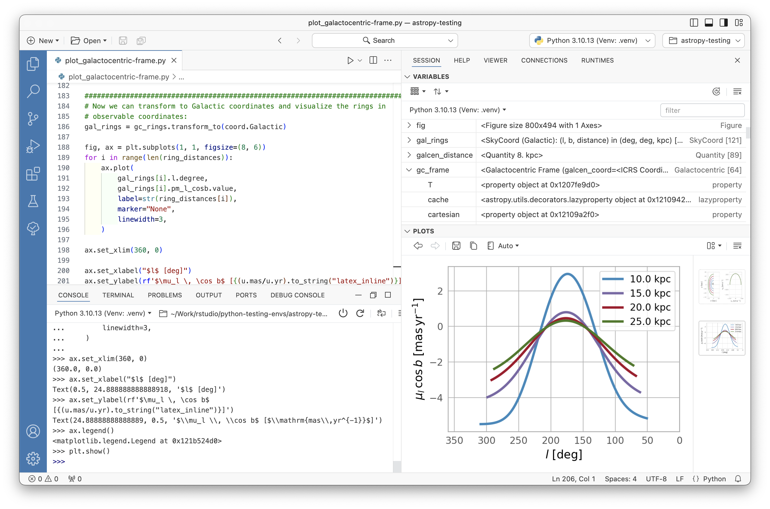
Positron

Sometimes Python is not so easy to setup. In addition is not as interactive as R (i.e., line by line evaluation). Posit (ex. R Studio) recently created Positron that is a new IDE working with R and Python at the same way.

Modern R

For purist programmers, R is weird: arrays starts with 1, object-oriented programming is hidden, a lot of built-in vectorized functions, etc. The The R Inferno book is really funny showing the strange R-stuff.
Despite the weirdness, R is widely used because it is intuitive (for non-programmers) and made for statistics and data manipulation
R is a language and as in spoken languages you can elegant, rude, ambiguous, funny, etc.
There are some tips to improve the readability and reproducibility of your code

Functional Programming

In computer science, functional programming is a programming paradigm where programs are constructed by applying and composing functions.

Despite R can be used both with an imperative and object-oriented approach, the functional side is quite powerful.
The basic idea is to decompose your code into small, testable and re-usable functions

Functional Programming, example…

We have a dataset (mtcars) and we want to calculate the mean, median, standard deviation, minimum and maximum of each column and store the result in a table.

head(mtcars)

#>                    mpg cyl disp  hp drat    wt  qsec vs am gear carb
#> Mazda RX4         21.0   6  160 110 3.90 2.620 16.46  0  1    4    4
#> Mazda RX4 Wag     21.0   6  160 110 3.90 2.875 17.02  0  1    4    4
#> Datsun 710        22.8   4  108  93 3.85 2.320 18.61  1  1    4    1
#> Hornet 4 Drive    21.4   6  258 110 3.08 3.215 19.44  1  0    3    1
#> Hornet Sportabout 18.7   8  360 175 3.15 3.440 17.02  0  0    3    2
#> Valiant           18.1   6  225 105 2.76 3.460 20.22  1  0    3    1

str(mtcars)

#> 'data.frame':    32 obs. of  11 variables:
#>  $ mpg : num  21 21 22.8 21.4 18.7 18.1 14.3 24.4 22.8 19.2 ...
#>  $ cyl : num  6 6 4 6 8 6 8 4 4 6 ...
#>  $ disp: num  160 160 108 258 360 ...
#>  $ hp  : num  110 110 93 110 175 105 245 62 95 123 ...
#>  $ drat: num  3.9 3.9 3.85 3.08 3.15 2.76 3.21 3.69 3.92 3.92 ...
#>  $ wt  : num  2.62 2.88 2.32 3.21 3.44 ...
#>  $ qsec: num  16.5 17 18.6 19.4 17 ...
#>  $ vs  : num  0 0 1 1 0 1 0 1 1 1 ...
#>  $ am  : num  1 1 1 0 0 0 0 0 0 0 ...
#>  $ gear: num  4 4 4 3 3 3 3 4 4 4 ...
#>  $ carb: num  4 4 1 1 2 1 4 2 2 4 ...

Functional Programming

The standard (~imperative) option is using a for loop, iterating through columns, calculate the values and store into another data structure.

ncols <- ncol(mtcars)
means <- medians <- mins <- maxs <- rep(0, ncols)

for(i in 1:ncols){
  means[i] <- mean(mtcars[[i]])
  medians[i] <- median(mtcars[[i]])
  mins[i] <- min(mtcars[[i]])
  maxs[i] <- max(mtcars[[i]])
}

results <- data.frame(means, medians, mins, maxs)
results$col <- names(mtcars)

results

#>         means medians   mins    maxs  col
#> 1   20.090625  19.200 10.400  33.900  mpg
#> 2    6.187500   6.000  4.000   8.000  cyl
#> 3  230.721875 196.300 71.100 472.000 disp
#> 4  146.687500 123.000 52.000 335.000   hp
#> 5    3.596563   3.695  2.760   4.930 drat
#> 6    3.217250   3.325  1.513   5.424   wt
#> 7   17.848750  17.710 14.500  22.900 qsec
#> 8    0.437500   0.000  0.000   1.000   vs
#> 9    0.406250   0.000  0.000   1.000   am
#> 10   3.687500   4.000  3.000   5.000 gear
#> 11   2.812500   2.000  1.000   8.000 carb

Functional Programming

The main idea is to decompose the problem writing a function and loop over the columns of the dataframe:

summ <- function(x){
  data.frame(means = mean(x), 
             medians = median(x), 
             mins = min(x), 
             maxs = max(x))
}
ncols <- ncol(mtcars)
dfs <- vector(mode = "list", length = ncols)

for(i in 1:ncols){
  dfs[[i]] <- summ(mtcars[[i]])
}

Functional Programming

results <- do.call(rbind, dfs)
results

#>         means medians   mins    maxs
#> 1   20.090625  19.200 10.400  33.900
#> 2    6.187500   6.000  4.000   8.000
#> 3  230.721875 196.300 71.100 472.000
#> 4  146.687500 123.000 52.000 335.000
#> 5    3.596563   3.695  2.760   4.930
#> 6    3.217250   3.325  1.513   5.424
#> 7   17.848750  17.710 14.500  22.900
#> 8    0.437500   0.000  0.000   1.000
#> 9    0.406250   0.000  0.000   1.000
#> 10   3.687500   4.000  3.000   5.000
#> 11   2.812500   2.000  1.000   8.000

Functional Programming

The actual real functional way require using the built-in iteration tools *apply. In this way you avoid writing the verbose for loop.

results <- lapply(mtcars, summ)
results <- do.call(rbind, results)
results

#>           means medians   mins    maxs
#> mpg   20.090625  19.200 10.400  33.900
#> cyl    6.187500   6.000  4.000   8.000
#> disp 230.721875 196.300 71.100 472.000
#> hp   146.687500 123.000 52.000 335.000
#> drat   3.596563   3.695  2.760   4.930
#> wt     3.217250   3.325  1.513   5.424
#> qsec  17.848750  17.710 14.500  22.900
#> vs     0.437500   0.000  0.000   1.000
#> am     0.406250   0.000  0.000   1.000
#> gear   3.687500   4.000  3.000   5.000
#> carb   2.812500   2.000  1.000   8.000

Functional Programming, `*apply`

The *apply family is one of the best tool in R. The idea is pretty simple: apply a function to each element of a list.
The powerful side is that in R everything can be considered as a list. A vector is a list of single elements, a dataframe is a list of columns etc.
Internally, R is still using a for loop but the verbose part (preallocation, choosing the iterator, indexing) is encapsulated into the *apply function.

means <- rep(0, ncol(mtcars))
for(i in 1:length(means)){
  means[i] <- mean(mtcars[[i]])
}

# the same with sapply
means <- sapply(mtcars, mean)

`for` loops are bad?

for loops are the core of each operation in R (and in every programming language). For complex operation thery are more readable and effective compared to *apply. In R we need extra care for writing efficent for loops.

Extremely slow, no preallocation:

res <- c()
for(i in 1:1000){
  # do something
  res[i] <- x
}

Very fast, no difference compared to *apply

res <- rep(0, 1000)
for(i in 1:length(res)){
  # do something
  res[i] <- x
}

`for` loops are bad?

We can formally compare the for loop approaches using the microbenchmark package:

no_prealloc <- function(n = 100){
    res <- c()
    for(i in 1:n) res[i] <- rnorm(1)
}

prealloc <- function(n = 100){
    res <- vector(mode = "numeric", length = n)
    for(i in 1:n) res[i] <- rnorm(1)
}

microbenchmark::microbenchmark(
    no_prealloc = no_prealloc(1000),
    prealloc = prealloc(1000)
)

#> Unit: microseconds
#>         expr     min       lq      mean   median       uq      max neval cld
#>  no_prealloc 848.225 872.0795 1010.1748 884.2175 918.5970 4462.520   100  a 
#>     prealloc 648.589 663.1315  711.0051 668.4970 681.6215 2821.114   100   b

`for` loops are bad?

In fact, when the for loop is written appropriately, the performance are the same (or even better) compared to *apply:

library(purrr) # for map
iter <- 500

microbenchmark::microbenchmark(
    for_no_prealloc = no_prealloc(iter),
    for_prealloc = prealloc(iter),
    sapply = sapply(1:iter, function(x) rnorm(1)),
    map_dbl = map_dbl(1:iter, function(x) rnorm(1)),
    vapply = vapply(1:iter, function(x) rnorm(1), FUN.VALUE = double(1)),
    times = 500
) |> summary()

#>              expr     min       lq     mean   median       uq      max neval
#> 1 for_no_prealloc 427.404 444.7960 479.5039 452.2905 463.0960 4068.079   500
#> 2    for_prealloc 321.355 330.5470 347.4882 334.3735 339.7890 4380.626   500
#> 3          sapply 588.496 607.2065 652.3096 618.3775 633.7065 5153.349   500
#> 4         map_dbl 610.588 630.8610 697.8509 645.0725 679.1320 4740.082   500
#> 5          vapply 579.730 591.2970 635.9248 598.4200 607.1715 4754.439   500
#>    cld
#> 1 a   
#> 2  b  
#> 3   cd
#> 4   c 
#> 5    d

With `*apply` you can do crazy stuff!

funs <- list(mean = mean, sd = sd, min = min, max = max, median = median)
sapply(funs, function(f) lapply(mtcars, function(x) f(x)))

#>      mean     sd        min   max   median
#> mpg  20.09062 6.026948  10.4  33.9  19.2  
#> cyl  6.1875   1.785922  4     8     6     
#> disp 230.7219 123.9387  71.1  472   196.3 
#> hp   146.6875 68.56287  52    335   123   
#> drat 3.596563 0.5346787 2.76  4.93  3.695 
#> wt   3.21725  0.9784574 1.513 5.424 3.325 
#> qsec 17.84875 1.786943  14.5  22.9  17.71 
#> vs   0.4375   0.5040161 0     1     0     
#> am   0.40625  0.4989909 0     1     0     
#> gear 3.6875   0.7378041 3     5     4     
#> carb 2.8125   1.6152    1     8     2

Why functional programming?

We can write less and reusable code that can be shared and used in multiple projects
The scripts are more compact, easy to modify and less error prone (imagine that you want to improve the summ function, you only need to change it once instead of touching the for loop)
Functions can be easily and consistently documented (see roxygen documentation) improving the reproducibility and readability of your code

More about functional programming in R

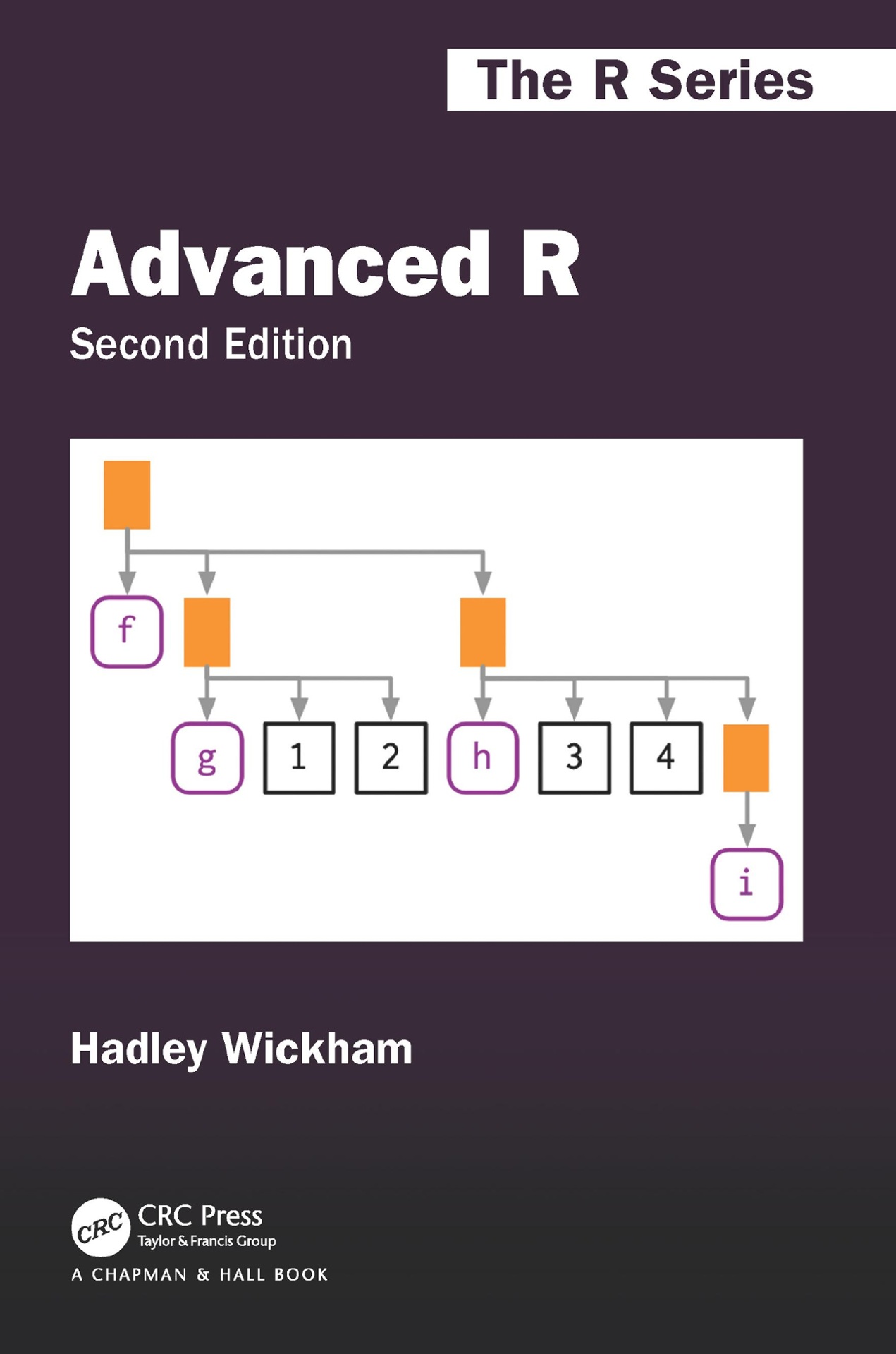
Advanced R by Hadley Wickham, section on Functional Programming (https://adv-r.hadley.nz/fp.html)
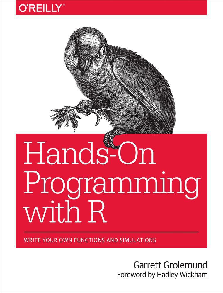
Hands-On Programming with R by Garrett Grolemund https://rstudio-education.github.io/hopr/
Hadley Wickham: The Joy of Functional Programming (for Data Science)
Bruno Rodrigues Youtube Channel

Advanced R Hands-on Programming With R

A small example

Take the dataset iris and do the following operations in the most readable and efficient way that you can.

fit a linear model (choose the y and x that you want) for each Species on the full dataset
fit a linear model (choose the y and x that you want) for each Species but resampling with replacement (bootstrapping, choose the number of iterations that you want) the rows within each group
(choose the y and x that you want) for each Species doing a leave-one-out analysis within each group
organize the three steps into separated datasets in a nice and readable format (nice column names, not strange characters, spaces, etc.)
show the results with a plot of your choice

A more advanced approach, R packages

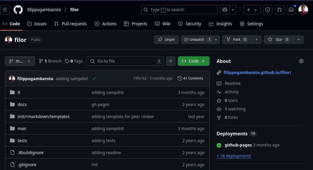
R packages are not only on CRAN. You can (pretty) easily create a package and put it on Github. For example, if you keep using some functions in your project, write a general version and put them into a package.

github.com/filippogambarota/filor

A more advanced approach, R packages

If your functions are project-specific you can define them into your scripts or write some R scripts only with functions and source() them into the global environment.

project/
├─ R/
│  ├─ utils.R
├─ analysis.R

And inside utils.R you have some functions:

myfun <- function(x) {
  # something
}

Then you can load the function using source("R/utils.R) at the beginning of analysis.R:

source("R/utils.R")

Analysis project as R package

The R project structure is really interesting to organize a data analysis pipeline. In fact, you can use the project structure. Vuorre and Crump (2021) and Marwick, Boettiger, and Mullen (2018) describe in details the idea.

The general approach is:

Create an R Studio project .Rproj file
Create your directories, put scripts, data, etc.
Create an R/ folder and put your scripts with functions
Create a DESCRIPTION file using usethis::use_description(check_name = FALSE)
Then you can load your functions without source and with devtools::load_all() (same as library())

Let’s see an example!

The Tidy approach

The tidyverse is a series of high-quality R packages to do modern data science:

data manipulation (dplyr, tidyr)
plotting (ggplot2)
reporting (rmarkdown)
string manipulation (stringr)
functionals (purrr)
…

The Tidy approach - Pipes

One of the great improvement from the tidyverse is the usage of the pipe %>% now introduced in base R as |>. You will se these symbols a lot when looking at modern R code.

The idea is very simple, the standard pattern to apply a function is function(argument). The pipe can reverse the pattern as argument |> function(). Normally when we apply multiple functions progressively the pattern is this:

x <- rnorm(100)
x <- round(x, 3)
x <- abs(x)
x <- as.character(x)

The Tidy approach - Pipes

When using the pipe, we remove the redundand assignment <- pattern:

x <- rnorm(100)
x |>
  round(3) |>
  abs() |>
  as.character()

The pipe can be read as “from x apply round, then abs, etc.”. The first argument of the piped function is assumed to be the result of the previus call.

More about the Tidy approach

The tidy approach contains tons of functions and packages. The overall philosophy can be deepen in the R for Data Science book.

https://r4ds.hadley.nz/

ggplot2

Only an quick mention to ggplot2 https://ggplot2-book.org/ (part of the tidyverse) that is an amazing package for data visualization following the piping and tidy approach. Is the implementation of the grammar of graphics idea.

library(tidyverse)

iris |>
  mutate(wi = runif(n())) |>
  ggplot(aes(x = Sepal.Length, y = Petal.Width, color = Species)) +
  geom_point(aes(size = wi)) +
  geom_smooth(method = "lm", se = FALSE)
  guides(size = "none") +
  theme_minimal(15)

ggplot2

Base R version

More verbose, more hard coding, more steps and intermediate objects.

iris_l <- split(iris, iris$Species)
lms <- lapply(iris_l, function(x) lm(Petal.Width ~ Sepal.Length, data = x))

plot(iris$Sepal.Length, 
     iris$Petal.Width, 
     col = as.numeric(iris$Species), pch = 19)

abline(lms[[1]], col = 1, lwd = 2)
abline(lms[[2]], col = 2, lwd = 2)
abline(lms[[3]], col = 3, lwd = 2)

legend("topleft", legend = levels(iris$Species), fill = 1:3)

Base R version

More on ggplot2

The ggplot2 book https://ggplot2-book.org/ is a great resource to produce high-quality, publication ready plots. Clearly, the advantage of producing the figures entirely writing code are immense in terms of reusability and reproducibility.

Something crazy in the `tidyverse`

Without going into details, I want to show you a very interesting approach that you can do with the tidyverse functions.

Let’s assume you want to do a leave-one-out analysis thus fitting the same models on a dataset, removing one observation at time.

You can do it in base R with a loop or other methods, but the see so-called many-models approach. See https://r4ds.had.co.nz/many-models.html and https://www.youtube.com/watch?v=rz3_FDVt9eg.

Something crazy in the `tidyverse`

Let’s define some functions:

leave1out <- function(data){
  idx <- 1:nrow(data)
  ll <- lapply(idx, function(i) data[-i, ])
  names(ll) <- paste0("no", idx)
  c(no0 = list(data), ll)
}

fit_model <- function(data){
  lm(Sepal.Length ~ Petal.Width, data = data)
}

Something crazy in the `tidyverse`

dat <- tibble(data = leave1out(iris[1:20, ]))
dat |> 
  mutate(removed = names(data)) |> 
  head()

#> # A tibble: 6 × 2
#>   data          removed
#>   <named list>  <chr>  
#> 1 <df [20 × 5]> no0    
#> 2 <df [19 × 5]> no1    
#> 3 <df [19 × 5]> no2    
#> 4 <df [19 × 5]> no3    
#> 5 <df [19 × 5]> no4    
#> 6 <df [19 × 5]> no5

Something crazy in the `tidyverse`

#> # A tibble: 6 × 4
#>   data          removed fit          results         
#>   <named list>  <chr>   <named list> <named list>    
#> 1 <df [20 × 5]> no0     <lm>         <tibble [2 × 5]>
#> 2 <df [19 × 5]> no1     <lm>         <tibble [2 × 5]>
#> 3 <df [19 × 5]> no2     <lm>         <tibble [2 × 5]>
#> 4 <df [19 × 5]> no3     <lm>         <tibble [2 × 5]>
#> 5 <df [19 × 5]> no4     <lm>         <tibble [2 × 5]>
#> 6 <df [19 × 5]> no5     <lm>         <tibble [2 × 5]>

Something crazy in the `tidyverse`

dat |> 
  mutate(removed = names(data)) |> 
  mutate(fit = map(data, fit_model),
         results = map(fit, broom::tidy)) |> 
  unnest(results) |> 
  ggplot(aes(x = removed, y = estimate)) +
  geom_point() +
  geom_line() +
  facet_wrap(~term, scales = "free")

Something crazy in the `tidyverse`

Quick tables

Characteristic	N = 150¹
Sepal.Length	5.80 (5.10, 6.40)
Sepal.Width	3.00 (2.80, 3.30)
Petal.Length	4.35 (1.60, 5.10)
Petal.Width	1.30 (0.30, 1.80)
Species
setosa	50 (33%)
versicolor	50 (33%)
virginica	50 (33%)
¹ Median (IQR); n (%)

Quick tables from models

fit <- lm(Sepal.Length ~ Petal.Width, data = iris)
sjPlot::tab_model(fit)

	Sepal.Length
Predictors	Estimates	CI	p
(Intercept)	4.78	4.63 – 4.92	<0.001
Petal Width	0.89	0.79 – 0.99	<0.001
Observations	150
R² / R² adjusted	0.669 / 0.667

Quick tables from models

gtsummary::tbl_regression(fit)

Characteristic	Beta	95% CI¹	p-value
Petal.Width	0.89	0.79, 0.99	<0.001
¹ CI = Confidence Interval

References

Marwick, Ben, Carl Boettiger, and Lincoln Mullen. 2018. “Packaging Data Analytical Work Reproducibly Using r (and Friends).” The American Statistician 72 (January): 80–88. https://doi.org/10.1080/00031305.2017.1375986.

Vuorre, Matti, and Matthew J C Crump. 2021. “Sharing and Organizing Research Products as r Packages.” Behavior Research Methods 53 (April): 792–802. https://doi.org/10.3758/s13428-020-01436-x.

Modern R

Reproducibility starter pack

Reproducibility starter pack 👷

Disclaimers

R Programming Language

R

R - CRAN

R - PYPL Index

R - PYPL Index

R or Python?

Positron

Modern R

Functional Programming

Functional Programming, example…

Functional Programming

Functional Programming

Functional Programming

Functional Programming

Functional Programming, *apply

for loops are bad?

for loops are bad?

for loops are bad?

With *apply you can do crazy stuff!

Why functional programming?

More about functional programming in R

A small example

A small example

A more advanced approach, R packages

A more advanced approach, R packages

Analysis project as R package

Let’s see an example!

The Tidy approach

The Tidy approach - Pipes

The Tidy approach - Pipes

More about the Tidy approach

ggplot2

ggplot2

Base R version

Base R version

More on ggplot2

Something crazy in the tidyverse

Something crazy in the tidyverse

Something crazy in the tidyverse

Something crazy in the tidyverse

Something crazy in the tidyverse

Something crazy in the tidyverse

Quick tables

Quick tables from models

Quick tables from models

References

Functional Programming, `*apply`

`for` loops are bad?

`for` loops are bad?

`for` loops are bad?

With `*apply` you can do crazy stuff!

Something crazy in the `tidyverse`

Something crazy in the `tidyverse`

Something crazy in the `tidyverse`

Something crazy in the `tidyverse`

Something crazy in the `tidyverse`

Something crazy in the `tidyverse`