Power analysis
Psicometria per le Neuroscienze Cognitive
Filippo Gambarota, PhD
Statistical Power
Power in a nutshell1
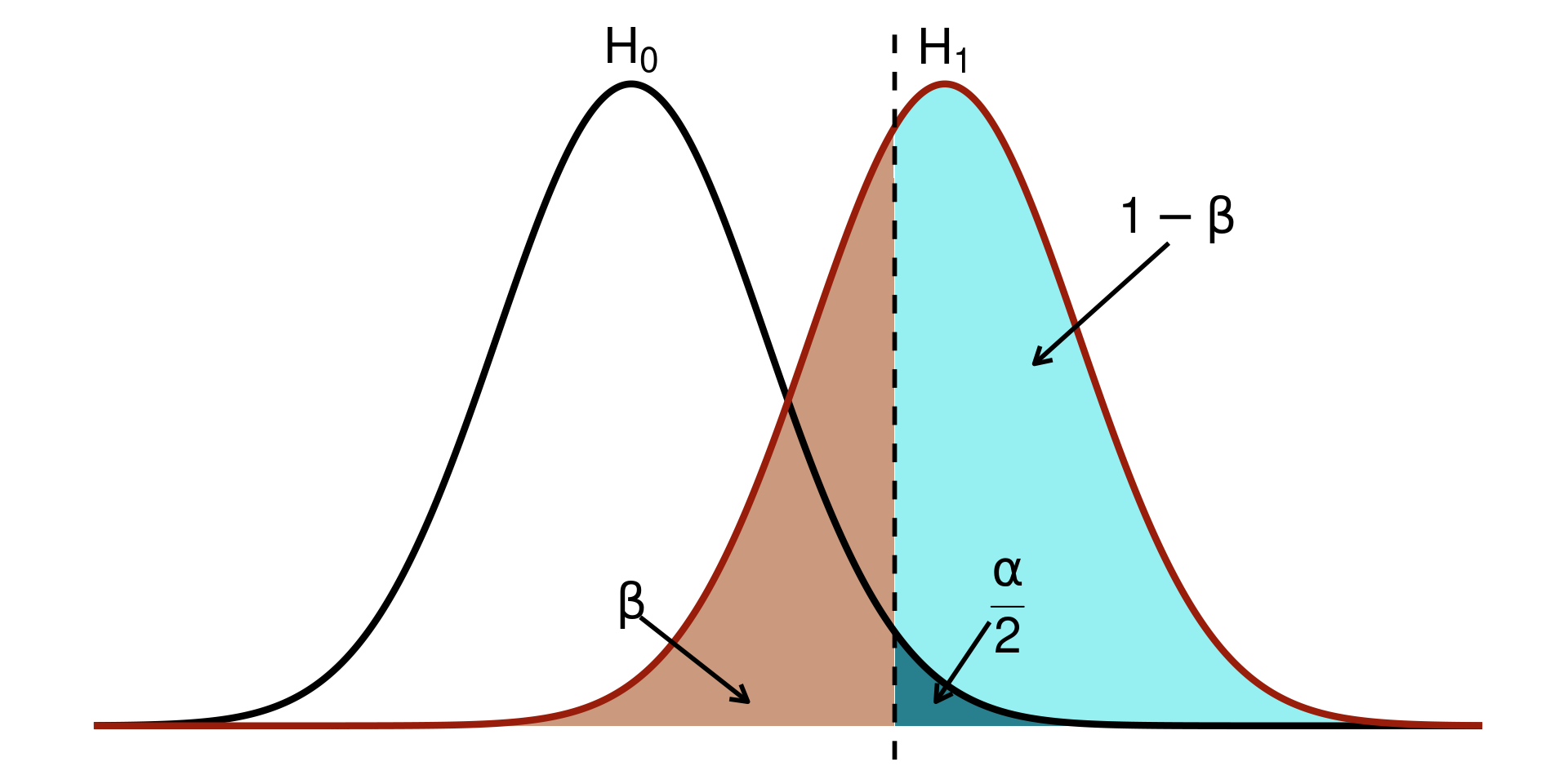
The stastistical power is defined as the probability of correctly rejecting the null hypothesis \(H_0\).
Power in a nutshell
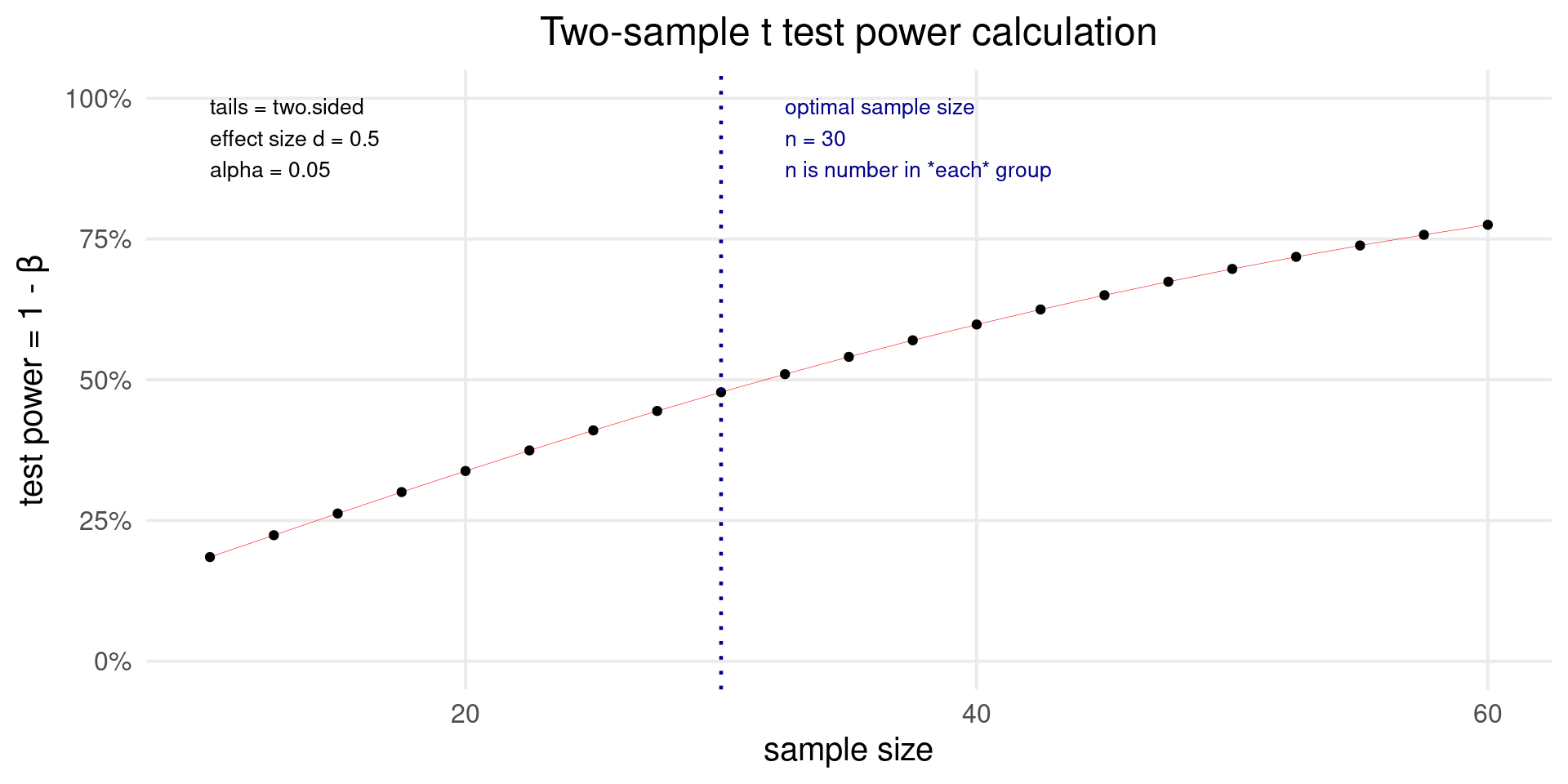
For simple designs such as t-test, ANOVA, etc. the power can be computed analytically. For example, let’s find the power of detecting an effect size of \(d = 0.5\) with \(n1 = n2 = 30\).
d <- 0.5
alpha <- 0.05
n1 <- n2 <- 30
sp <- 1

# Calculate non-centrality parameter (delta)
delta <- d * sqrt(n1 * n2 / (n1 + n2))

# Calculate degrees of freedom
df <- n1 + n2 - 2

# Calculate critical t-value
critical_t <- qt(1 - alpha / 2, df)

# Calculate non-central t-distribution value
non_central_t <- delta / sp

# Calculate power
1 - pt(critical_t - non_central_t, df)
#> [1] 0.4741093
Power in a nutshell
The same can be done using the pwr package:
Power in a nutshell
Power by simulations
Sometimes the analytical solution is not available or we can estimate the power for complex scenarios (missing data, unequal variances, etc.). The general workflow is:
- Generate data under the parametric assumptions
- Fit the appropriate model
- Extract the relevant metric (e.g., p-value)
- Repeat 1-3 several times (1000, 10000 or more)
- Summarise the results
For example, the power is the number of p-values lower than \(\alpha\) over the total number of simulations.
Power by simulations
Let’s see the previous example using simulations:
The estimated value is pretty close to the analytical value.
What about meta-analysis
Also for meta-analysis we have the two approaches analytical and simulation-based.
Analytical approach
For the analytical approach we need to make some assumptions:
- \(\tau^2\) and \(\mu_{\theta}\) (or \(\theta\)) are estimated without errors
- The \(\sigma^2_i\) (thus the sample size) of each \(k\) study is the same
Under these assumptions the power is:
\[ (1 - \Phi(c_{\alpha} - \lambda)) + \Phi(-c_{\alpha} - \lambda) \]
Where \(c_{\alpha}\) is the critical \(z\) value and \(\lambda\) is the observed statistics.
Analytical approach - EE model
For an EE model the only source of variability is the sampling variability, thus \(\lambda\):
\[ \lambda_{EE} = \frac{\theta}{\sqrt{\sigma^2_{\theta}}} \]
And recalling previous assuptions where \(\sigma^2_1 = \dots = \sigma^2_k\):
\[ \sigma^2_{\theta} = \frac{\sigma^2}{k} \]
Analytical approach - EE model
For example, a meta-analysis of \(k = 15\) studies where each study have a sample size of \(n1 = n2 = 20\) (assuming again unstandardized mean difference as effect size):
Be careful that the EE model is assuming \(\tau^2 = 0\) thus is like having a huge study with \(k \times n_1\) participants per group.
Analytical approach - RE model
For the RE model we just need to include \(\tau^2\) in the \(\lambda\) calculation, thus:
\[ \sigma^{2\star}_{\theta} = \frac{\sigma^2 + \tau^2}{k} \]
The other calculations are the same as the EE model.
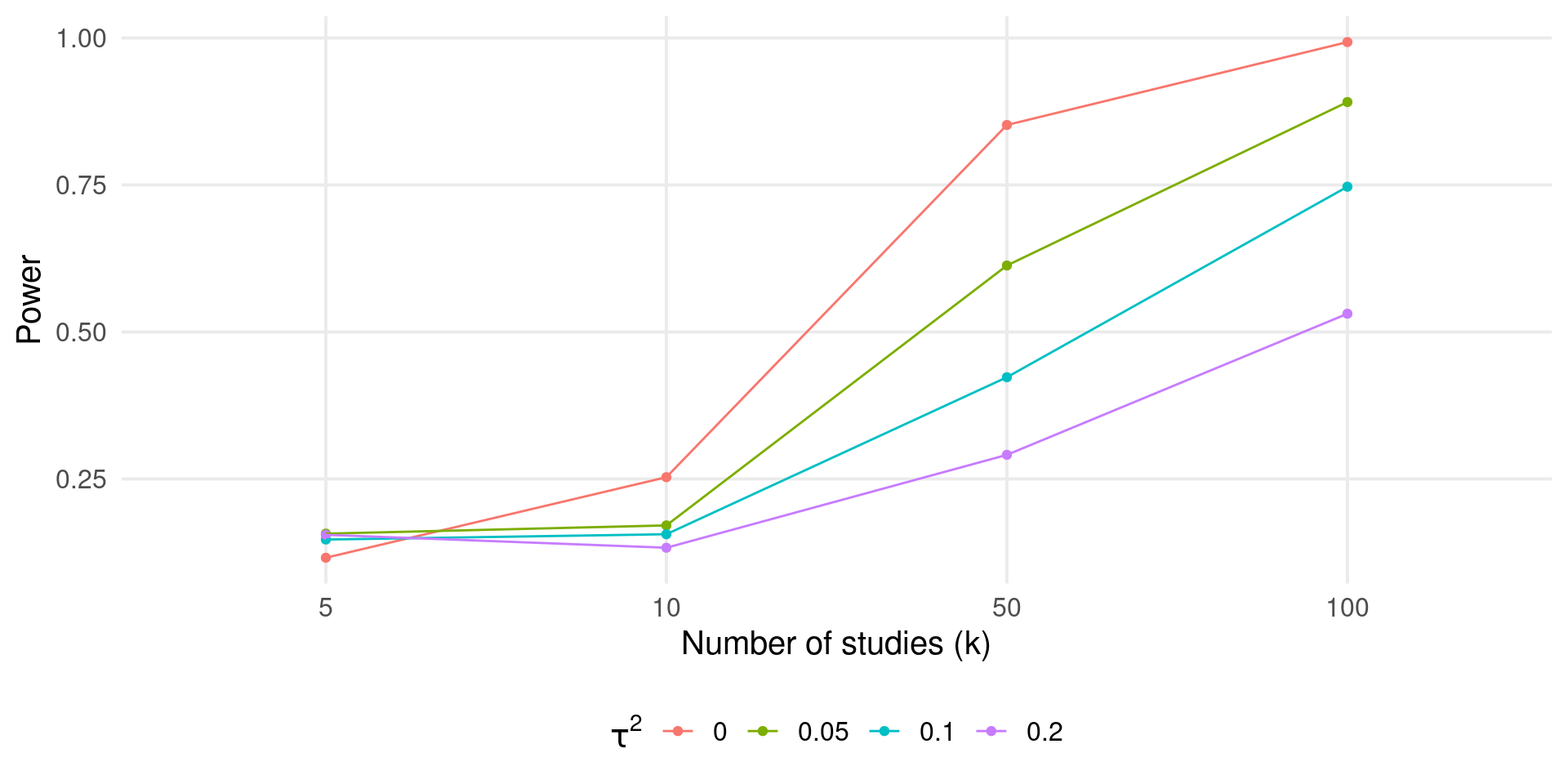
Analytical approach - RE model
The power is reduced because we are considering another source of heterogeneity. Clearly the maximal power of \(k\) studies is achieved when \(\tau^2 = 0\). Hypothetically we can increase the power either increasing \(k\) (the number of studies) or reducing \(\sigma^2_k\) (increasing the number of participants in each study).
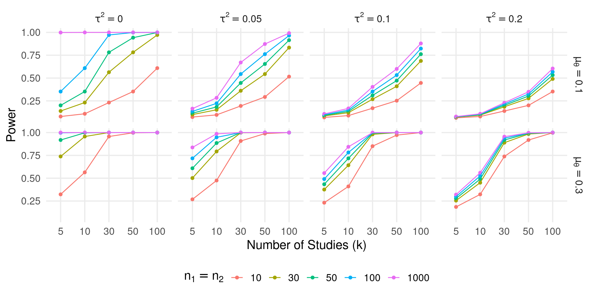
Analytical approach - Power curves
The most informative approach is plotting the power curves for different values of \(\tau^2\), \(\sigma^2_k\) and \(\theta\) (or \(\mu_{\theta}\)).
You can use the power_meta() function:
Analytical approach - Power curves
Code
k <- c(5, 10, 30, 50, 100)
es <- c(0.1, 0.3)
tau2 <- c(0, 0.05, 0.1, 0.2)
n <- c(10, 30, 50, 100, 1000)

power <- expand_grid(es, k, tau2, n1 = n)
power$power <- power_meta(power$es, power$k, power$tau2, power$n1)

power$es <- factor(power$es, labels = latex2exp::TeX(sprintf("$\\mu_{\\theta} = %s$", es)))
power$tau2 <- factor(power$tau2, labels = latex2exp::TeX(sprintf("$\\tau^2 = %s$", tau2)))

ggplot(power, aes(x = factor(k), y = power, color = factor(n1))) +
  geom_point() +
  geom_line(aes(group = factor(n1))) +
  facet_grid(es~tau2, labeller = label_parsed) +
  xlab("Number of Studies (k)") +
  ylab("Power") +
  labs(
    color = latex2exp::TeX("$n_1 = n_2$")
  )
Analytical approach - Power curves
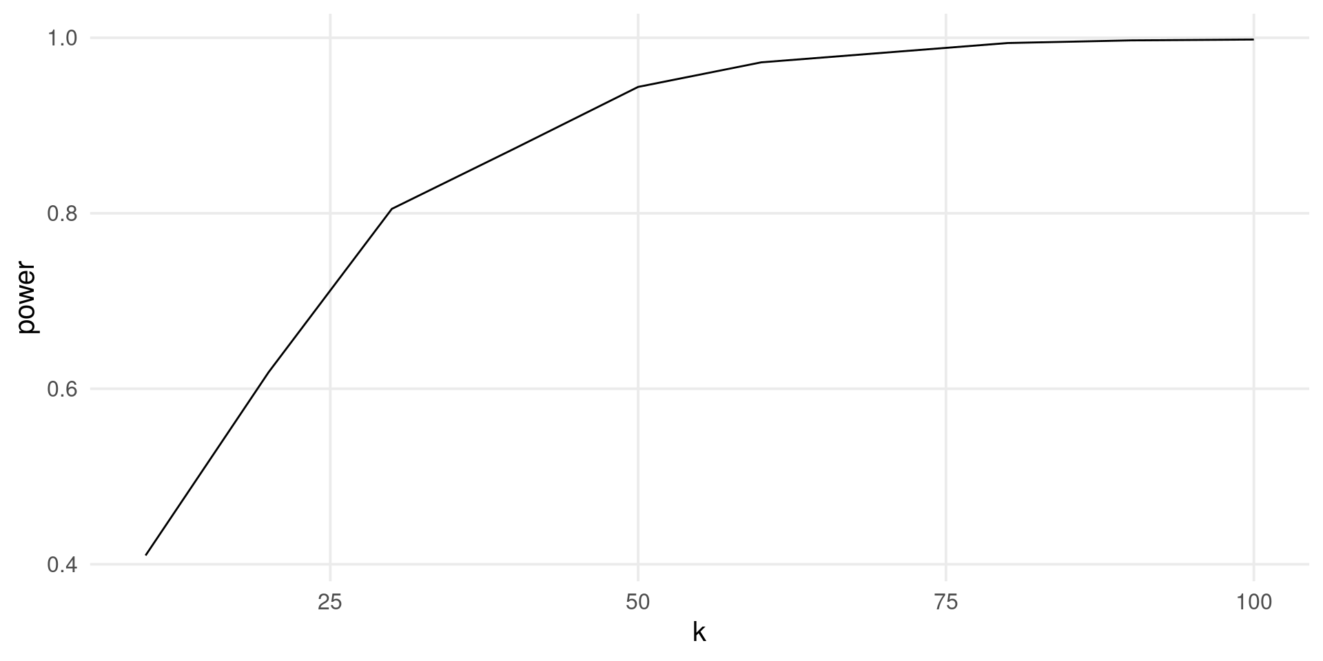
With the analytical approach we can (quickly) do interesting stuff. For example, we fix the total \(N = n_1 + n_2\) for a series of \(k\) and check the power.
Code
# average meta k = 20, n = 30
kavg <- 20
navg <- 30
N <- kavg * (navg*2)
es <- 0.3
tau2 <- c(0, 0.05, 0.1, 0.2)
k <- seq(10, 100, 10)
n1 <- n2 <- round((N/k)/ 2)

sim <- data.frame(es, k, n1, n2)
sim <- expand_grid(sim, tau2 = tau2)
sim$power <- power_meta(sim$es, sim$k, sim$tau2, sim$n1, sim$n2)
sim$N <- with(sim, k * (n1 + n2))

ggplot(sim, aes(x = k, y = power, color = factor(tau2))) +
  geom_line() +
  ggtitle(latex2exp::TeX("Total N ($n_1 + n_2$) = 1200")) +
  labs(x = "Number of Studies (k)",
       y = "Power",
       color = latex2exp::TeX("$\\tau^2$"))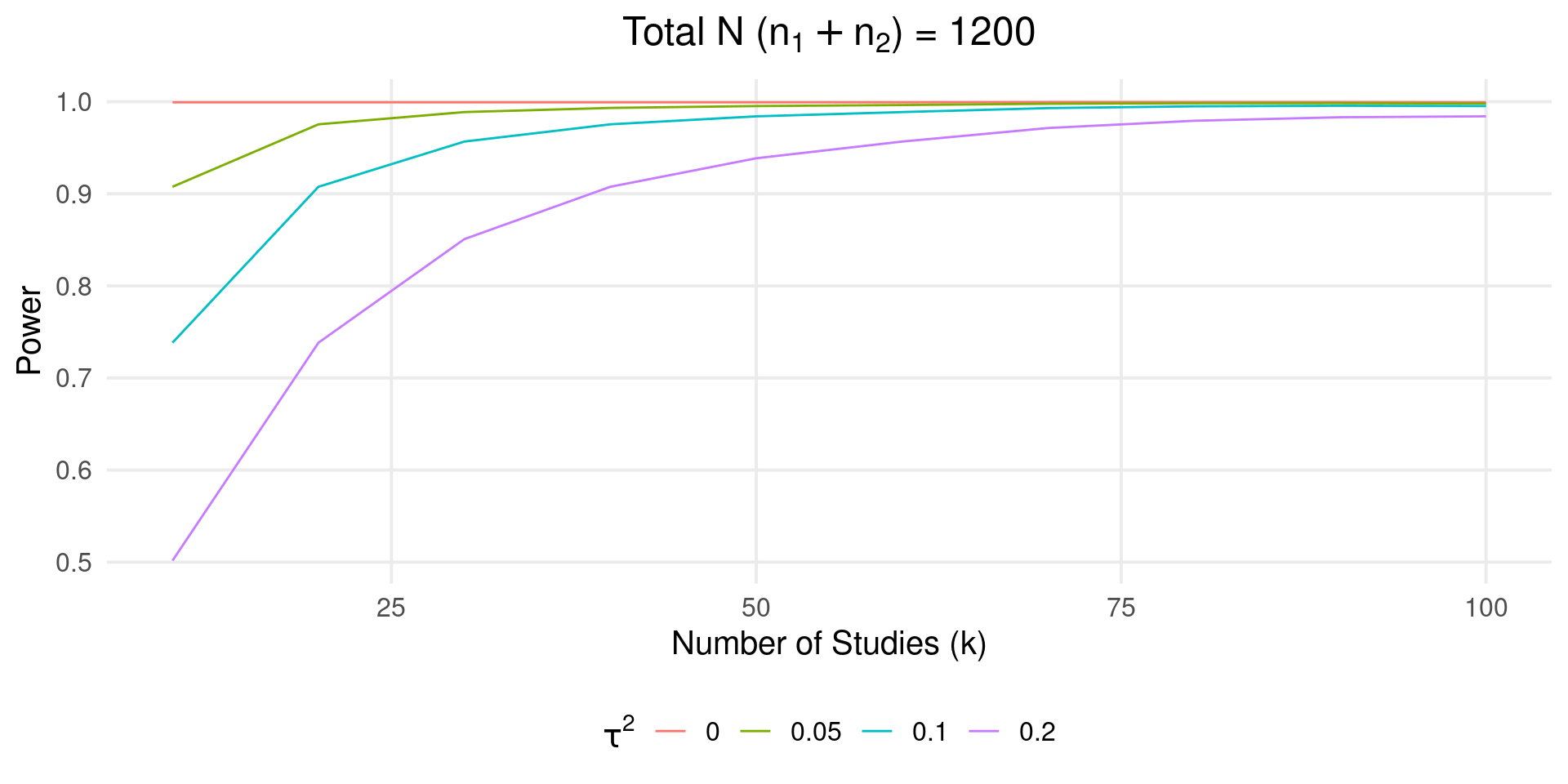
As long as \(\tau^2 \neq 0\) we need more studies (even if the total sample size is the same).
Simulation-based power
With simulations we can fix or relax the previous assumptions. For example, let’s compute the power for an EE model:
The value is similar to the analytical simulation. But we can improve it e.g. generating heterogeneous sample sizes.
Simulation-based power curve
By repeating the previous approach for a series of parameters we can easily draw a power curve:
k <- c(5, 10, 50, 100)
es <- 0.1
tau2 <- c(0, 0.05, 0.1, 0.2)
nsim <- 1000

grid <- expand_grid(k, es, tau2)
power <- rep(NA, nrow(grid))

for(i in 1:nrow(grid)){
  pval <- rep(NA, nsim)
  for(j in 1:nsim){
    n <- rpois(grid$k[i], 40)
    dat <- sim_studies(grid$k[i], grid$es[i], grid$tau2[i], n)
    fit <- rma(yi, vi, data = dat)
    pval[j] <- fit$pval
  }
  power[i] <- mean(pval <= 0.05)
}
grid$power <- power
Simulation-based power curve
Power analysis for meta-regression
The power for a meta-regression can be easily computed by simulating the moderator effect. For example, let’s simulate the effect of a binary predictor \(x\).
k <- seq(10, 100, 10)
b0 <- 0.2 # average of group 1
b1 <- 0.1 # difference between group 1 and 2
tau2r <- 0.2 # residual tau2
nsim <- 1000
power <- rep(NA, length(k))

for(i in 1:length(k)){
  es <- b0 + b1 * rep(0:1, each = k[i]/2)
  pval <- rep(NA, nsim)
  for(j in 1:nsim){
    n <- round(runif(k[i], 10, 100))
    dat <- sim_studies(k[i], es, tau2r, n)
    fit <- rma(yi, vi, data = dat)
    pval[j] <- fit$pval
  }
  power[i] <- mean(pval <= 0.05)
}
Power analysis for meta-regression
Then we can plot the results:
Multilab Studies
Multilab studies
Multilab studies can be seen as a meta-analysis that is planned (a prospective meta-analysis) compared to standard retrospective meta-analysis.
The statistical approach is (roughly) the same with the difference that we have control both on \(k\) (the number of experimental units) and \(n\) the sample size within each unit.
In multilab studies we have also the raw data (i.e., participant-level data) thus we can do more complex multilevel modeling.
Meta-analysis as multilevel model
Assuming that we have \(k\) studies with raw data available there is no need to aggregate, calculate the effect size and variances and then use an EE or RE model.
k <- 50
es <- 0.4
tau2 <- 0.1
n <- round(runif(k, 10, 100))
dat <- vector(mode = "list", k)
thetai <- rnorm(k, 0, sqrt(tau2))

for(i in 1:k){
  g1 <- rnorm(n[i], 0, 1)
  g2 <- rnorm(n[i], es + thetai[i], 1)
  d <- data.frame(id = 1:(n[i]*2), unit = i, y = c(g1, g2), group = rep(c(0, 1), each = n[i]))
  dat[[i]] <- d
}

dat <- do.call(rbind, dat)
ht(dat)
#>      id unit          y group
#> 1     1    1 -0.4359058     0
#> 2     2    1  1.5799758     0
#> 3     3    1  0.7015053     0
#> 4     4    1  0.1376932     0
#> 5     5    1 -1.7018263     0
#> 5257 63   50  1.0430772     1
#> 5258 64   50 -0.7878105     1
#> 5259 65   50 -0.4609004     1
#> 5260 66   50  1.5076526     1
#> 5261 67   50  0.9963187     1
#> 5262 68   50 -0.2518844     1
Meta-analysis as multilevel model
This is a simple multilevel model (pupils within classrooms or trials within participants). We can fit the model using lme4::lmer():
library(lme4)
fit_lme <- lmer(y ~ group + (1|unit), data = dat)
summary(fit_lme)
#> Linear mixed model fit by REML ['lmerMod']
#> Formula: y ~ group + (1 | unit)
#>    Data: dat
#>
#> REML criterion at convergence: 15282.1
#>
#> Scaled residuals:
#>     Min      1Q  Median      3Q     Max
#> -3.6473 -0.6764  0.0169  0.6663  3.5499
#>
#> Random effects:
#>  Groups   Name        Variance Std.Dev.
#>  unit     (Intercept) 0.03605  0.1899
#>  Residual             1.05226  1.0258
#> Number of obs: 5262, groups:  unit, 50
#>
#> Fixed effects:
#>              Estimate Std. Error t value
#> (Intercept) 0.0006038  0.0341201   0.018
#> group       0.3992543  0.0282823  14.117
#>
#> Correlation of Fixed Effects:
#>       (Intr)
#> group -0.414
Meta-analysis as multilevel model
Let’s do the same as a meta-analysis. Firstly we compute the effect sizes for each unit:
Meta-analysis as multilevel model
ht(datagg)
#>
#>    unit           m0          m1       sd0       sd1 n0 n1      yi     vi
#> 1     1 -0.067197098  0.40582612 0.9304467 1.0147085 42 42  0.4730 0.0451
#> 2     2 -0.091403369 -0.39447251 1.1524521 1.0145999 22 22 -0.3031 0.1072
#> 3     3 -0.003808028  0.16236294 0.9414775 0.7959424 20 20  0.1662 0.0760
#> 4     4  0.074297764  0.14426023 0.9656452 1.0081848 97 97  0.0700 0.0201
#> 5     5 -0.068813812  0.26518665 0.9798539 1.1045266 26 26  0.3340 0.0838
#> 45   45 -0.030328846  0.18885527 0.9490194 1.0119891 96 96  0.2192 0.0200
#> 46   46  0.076619304  0.24552547 1.0223705 0.8317036 37 37  0.1689 0.0469
#> 47   47 -0.123421255  0.80612492 0.8958121 1.2418829 41 41  0.9295 0.0572
#> 48   48 -0.012340409 -0.27712644 1.0127637 0.9681938 85 85 -0.2648 0.0231
#> 49   49  0.351899444 -0.08890696 0.9262625 1.0037785 46 46 -0.4408 0.0406
#> 50   50 -0.231551420  0.21903620 1.1221262 0.9182845 34 34  0.4506 0.0618
Meta-analysis as multilevel model
Then we can fit the model:
fit_rma <- rma(yi, vi, data = datagg)
fit_rma
#>
#> Random-Effects Model (k = 50; tau^2 estimator: REML)
#>
#> tau^2 (estimated amount of total heterogeneity): 0.1623 (SE = 0.0419)
#> tau (square root of estimated tau^2 value):      0.4028
#> I^2 (total heterogeneity / total variability):   81.04%
#> H^2 (total variability / sampling variability):  5.28
#>
#> Test for Heterogeneity:
#> Q(df = 49) = 260.7313, p-val < .0001
#>
#> Model Results:
#>
#> estimate      se    zval    pval   ci.lb   ci.ub
#>   0.3711  0.0647  5.7356  <.0001  0.2443  0.4979  ***
#>
#> ---
#> Signif. codes:  0 '***' 0.001 '**' 0.01 '*' 0.05 '.' 0.1 ' ' 1
Meta-analysis as multilevel modeling
Actually the results are very similar where the standard deviation of the intercepts of the lme4 model is \(\approx \tau\) and the group effect is the intercept of the rma model.
data.frame(
  b = c(fixef(fit_lme)[2], fit_rma$b),
  se = c(summary(fit_lme)$coefficients[2, 2], fit_rma$se),
  tau2 = c(as.numeric(VarCorr(fit_lme)[[1]]), fit_rma$tau2),
  model = c("lme4", "metafor")
)
#>               b         se       tau2   model
#> group 0.3992543 0.02828232 0.03604771    lme4
#>       0.3710964 0.06470033 0.16226242 metafor
Actually the two model are not exactly the same, especially when using only the aggregated data. See https://www.metafor-project.org/doku.php/tips:rma_vs_lm_lme_lmer.
Meta-analysis as multilevel modeling
To note, aggregating data and then computing a standard (non-weighted) model (sometimes this is done with trial-level data) is wrong and should be avoided. Using meta-analysis is clear that aggregating without taking into account the cluster (e.g., study or subject) precision is misleading.
dataggl <- datagg |>
  select(unit, m0, m1) |>
  pivot_longer(c(m0, m1), values_to = "y", names_to = "group")

summary(lmer(y ~ group + (1|unit), data = dataggl))
#> Linear mixed model fit by REML ['lmerMod']
#> Formula: y ~ group + (1 | unit)
#>    Data: dataggl
#>
#> REML criterion at convergence: 63.5
#>
#> Scaled residuals:
#>     Min      1Q  Median      3Q     Max
#> -2.5460 -0.5662 -0.1141  0.4252  4.0163
#>
#> Random effects:
#>  Groups   Name        Variance Std.Dev.
#>  unit     (Intercept) 0.0000   0.0000
#>  Residual             0.1034   0.3215
#> Number of obs: 100, groups:  unit, 50
#>
#> Fixed effects:
#>             Estimate Std. Error t value
#> (Intercept) 0.009959   0.045473   0.219
#> groupm1     0.365573   0.064309   5.685
#>
#> Correlation of Fixed Effects:
#>         (Intr)
#> groupm1 -0.707
#> optimizer (nloptwrap) convergence code: 0 (OK)
#> boundary (singular) fit: see help('isSingular')
Mulitlab sample size vs unit
When planning a multilab study there is an important decision between increasing the sample size within each unit (more effort for each lab) or recruiting more units with less participants per unit (more effort for the organization).
We could have the situation where the number of units \(k\) is fixed and we can only increase the sample size.
We can also simulate scenarios where some units collect all data while others did not complete the data collection.
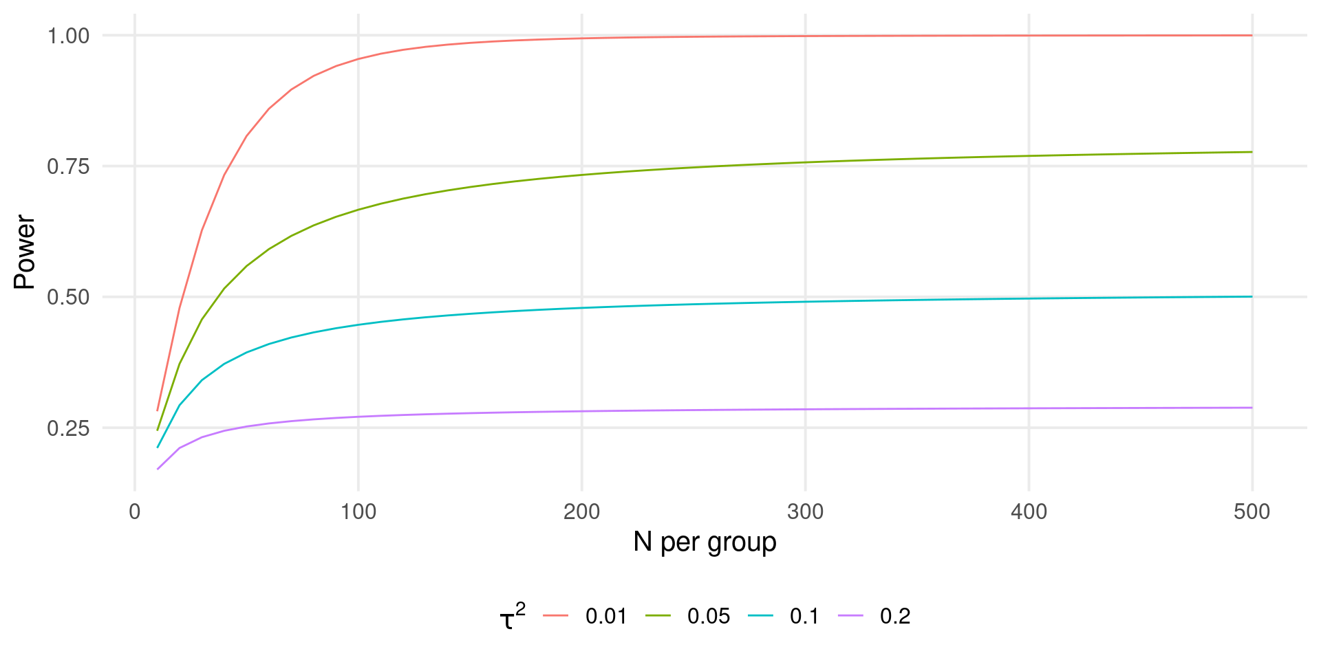
Fixed \(k\), increasing \(n\)
Let’s assume that the maximum number of labs is \(10\). How many participants are required assuming a certain amount of heterogeneity?
es <- 0.2
k <- 10
n1 <- n2 <- seq(10, 500, 10)
tau2 <- c(0.01, 0.05, 0.1, 0.2)
sim <- expand_grid(k, es, tau2, n1)
sim$n2 <- sim$n1
sim$vt <- with(sim, 1/n1 + 1/n2)
sim$I2 <- round(with(sim, tau2 / (tau2 + vt)) * 100, 3)
sim$power <- power_meta(sim$es, sim$k, sim$tau2, sim$n1, sim$n2)

ht(sim)
#> # A tibble: 11 × 8
#>        k    es  tau2    n1    n2      vt    I2 power
#>    <dbl> <dbl> <dbl> <dbl> <dbl>   <dbl> <dbl> <dbl>
#>  1    10   0.2  0.01    10    10 0.2      4.76 0.281
#>  2    10   0.2  0.01    20    20 0.1      9.09 0.479
#>  3    10   0.2  0.01    30    30 0.0667  13.0  0.627
#>  4    10   0.2  0.01    40    40 0.05    16.7  0.733
#>  5    10   0.2  0.01    50    50 0.04    20    0.807
#>  6    10   0.2  0.2    450   450 0.00444 97.8  0.288
#>  7    10   0.2  0.2    460   460 0.00435 97.9  0.288
#>  8    10   0.2  0.2    470   470 0.00426 97.9  0.288
#>  9    10   0.2  0.2    480   480 0.00417 98.0  0.288
#> 10    10   0.2  0.2    490   490 0.00408 98    0.288
#> 11    10   0.2  0.2    500   500 0.004   98.0  0.288
Fixed \(k\), increasing \(n\)
With a fixed \(k\), we could reach a plateau even increasing \(n\). This depends also on \(\mu_{\theta}\) and \(\tau^2\).
Multilab replication studies
A special type of multilab studies are the replication projects. There are some paper discussing how to view replication studies as meta-analyses and how to plan them.
References
Borenstein, Michael, Larry V Hedges, Julian P T Higgins, and Hannah R Rothstein. 2009. “Introduction to Meta-Analysis.” https://doi.org/10.1002/9780470743386.
Hedges, L V, and T D Pigott. 2001. “The Power of Statistical Tests in Meta-Analysis.” Psychological Methods 6 (September): 203–17. https://www.ncbi.nlm.nih.gov/pubmed/11570228.
Hedges, Larry V, and Jacob M Schauer. 2019. “Statistical Analyses for Studying Replication: Meta-Analytic Perspectives.” Psychological Methods 24 (October): 557–70. https://doi.org/10.1037/met0000189.
———. 2021. “The Design of Replication Studies.” Journal of the Royal Statistical Society. Series A, (Statistics in Society) 184 (July): 868–86. https://doi.org/10.1111/rssa.12688.
Jackson, Dan, and Rebecca Turner. 2017. “Power Analysis for Random-Effects Meta-Analysis.” Research Synthesis Methods 8 (September): 290–302. https://doi.org/10.1002/jrsm.1240.
Schauer, J M, and L V Hedges. 2021. “Reconsidering Statistical Methods for Assessing Replication.” Psychological Methods 26 (February): 127–39. https://doi.org/10.1037/met0000302.
Schauer, Jacob M. 2022. “Replicability and Meta-Analysis.” In Avoiding Questionable Research Practices in Applied Psychology, edited by William O’Donohue, Akihiko Masuda, and Scott Lilienfeld, 301–42. Cham: Springer International Publishing. https://doi.org/10.1007/978-3-031-04968-2_14.
———. 2023. “On the Accuracy of Replication Failure Rates.” Multivariate Behavioral Research 58 (May): 598–615. https://doi.org/10.1080/00273171.2022.2066500.
Schauer, Jacob M, and Larry V Hedges. 2020. “Assessing Heterogeneity and Power in Replications of Psychological Experiments.” Psychological Bulletin 146 (August): 701–19. https://doi.org/10.1037/bul0000232.
Valentine, Jeffrey C, Therese D Pigott, and Hannah R Rothstein. 2010. “How Many Studies Do You Need?: A Primer on Statistical Power for Meta-Analysis.” Journal of Educational and Behavioral Statistics: A Quarterly Publication Sponsored by the American Educational Research Association and the American Statistical Association 35 (April): 215–47. https://doi.org/10.3102/1076998609346961.