Probability of Replication

Probability of replication of a Binomial test for simple versus simple hypothesis. Inspired by Miller’s paper.

Model: \(x\) is Binomial \(\theta\). There are two possible values of \(\theta\) the null value \(\theta_0\) and the alternative \(\theta_1\). Both the original and replicated experiment have size \(n\). We know \(\gamma\).

The logic is this:

-- compute the power \((1-\beta\)) of the studies (it is the same for both) by simulation

-- for ever possible \(x\) in \(0, \ldots, n\) compute the p-value and the posterior probability of the null \(\theta=\theta_0\)

-- if the \(x\) leads to a rejection compute the probability of replication as \(\alpha/2 * p(\theta_0|x) + (1-\beta) (1-p(\theta_0|x))\)

-- if the \(x\) does not lead to a rejection compute the probability of replication as \((1-\alpha) * p(\theta_0|x) + \beta (1-p(\theta_0|x))\)

Function to compute the probability of replication.

probrep = function(
  nn, # sample size of both the initial and replication experiment
  gamma, # prior probability of the hypothesis
  theta0, # success probability under the null hypothesis
  theta1, # success probability under the null hypothesis
  alpha # significance cutoff
){
  x1range = seq(0,nn) # possible values of original experiment
  pvalue1 = pH0 = rep(NA,nn+1) # initialization
# type two error estimation via quick simulation
  MM = 10000
  xx.under.alt = rbinom(MM,nn,theta1)
  pvalue.alt = NA
  for (mm in 1:MM){
  pvalue.alt[mm] = binom.test(xx.under.alt[mm],nn,theta0,alternative="two.sided")$p.value
}
  beta = mean( pvalue.alt > .05) # type one error in both studies
#

for (xx in x1range){
# mapping between number of successes and pvalue in original ezxperiment
  pvalue1[xx] = 
    binom.test(xx,nn,theta0,alternative="two.sided")$p.value
# probability of null hypothesis given first experiment
  pH0[xx] = gamma * dbinom(xx,nn,theta0) / 
    ( gamma * dbinom(xx,nn,theta0) + (1-gamma) * dbinom(xx,nn,theta1))
}
# set tiny p-values to e-20 for visualization purposes
  pvalue1[is.na(pvalue1)] = 0
  pH0[is.na(pH0)] = 0
  # separate rejections 
  xx.reject = x1range[ pvalue1 < .05 ] + 1
  xx.retain = x1range[ pvalue1>=.05 ] + 1
  pvalue.reject = pvalue1[xx.reject]  
  pvalue.retain = pvalue1[xx.retain]
  pH0.reject = pH0[xx.reject]  
  pH0.retain = pH0[xx.retain]
  
#  browser()

  # compute replication probabilitie
  prep.reject = (alpha/2) * pH0[xx.reject] + (1-beta) * (1-pH0[xx.reject])
  prep.retain = (1-alpha) * pH0[xx.retain] + beta * (1-pH0[xx.retain])

  return(list(
    reject = na.omit(data.frame(prep.reject,pvalue.reject,pH0.reject)),
    retain = na.omit(data.frame(prep.retain,pvalue.retain,pH0.retain))))
}

probrep.out = probrep(nn=20,gamma=.5,theta0=.1,theta1=.2,alpha=0.05)
plot(probrep.out$reject$pvalue.reject,
     probrep.out$reject$prep.reject,
     ylab="probability of replication",
     xlab="p-value of original study")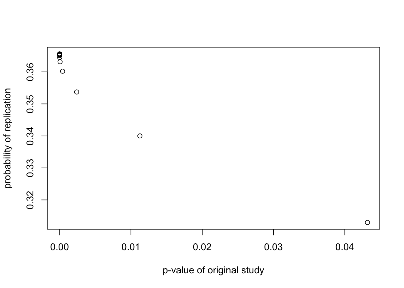

plot(probrep.out$reject$pvalue.reject,
     probrep.out$reject$pH0.reject,
     ylab="probability of null hypothesis",
     xlab="p-value of original study")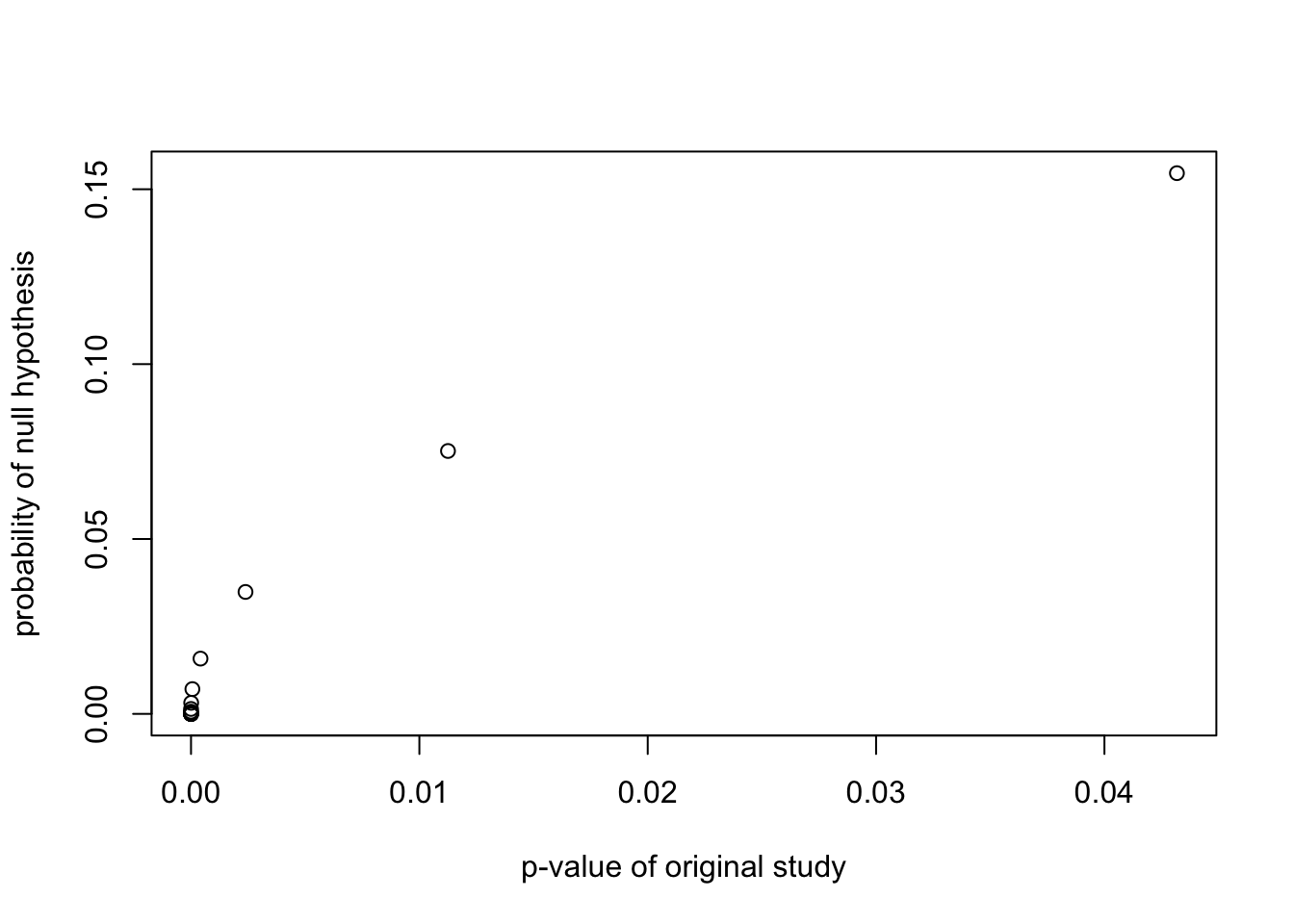

plot(probrep.out$retain$pvalue.retain,
     probrep.out$retain$prep.retain,
     ylab="probability of replication",
     xlab="p-value of original study")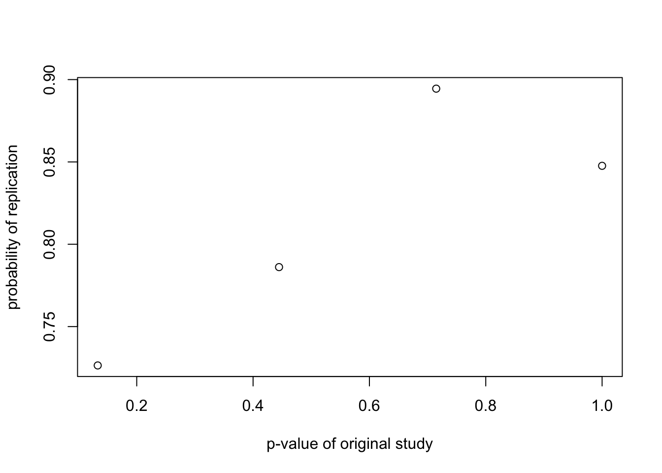

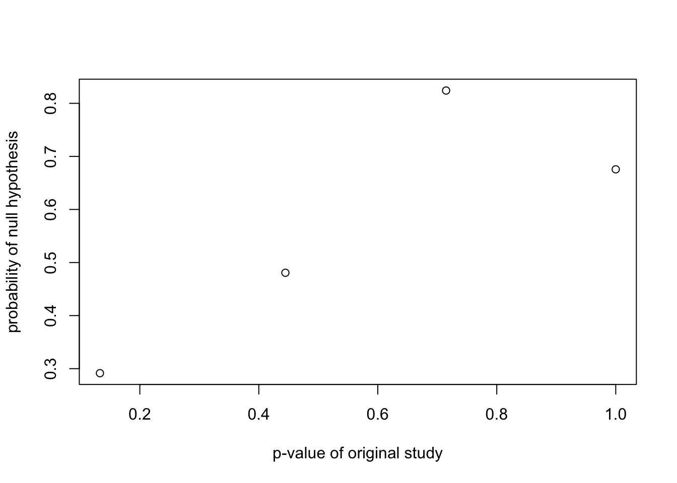
plot(probrep.out$retain$pvalue.retain,
     probrep.out$retain$pH0.retain,
     ylab="probability of null hypothesis",
     xlab="p-value of original study")