2025-04-07

Topics

Facciamo un’approfondimento su un’applicazione interessante del modello probit alle decisioni signal detection theory

Assignment

Per oggi facciamo una simulazione, descritta in questo documento

Simulazioni

Abbiamo visto alcune strategie di simulazione, in particolare per calcolare la potenza statistica. Ad esempio nel caso di un t-test assumendo due popolazioni a varianza uguale (\(\sigma = 1\)) e differenza tra le medie \(d = 0.3\) abbiamo:

n <- 30 # per gruppo
d <- 0.3 # effect size
s <- 1 # pooled standard deviation
df <- n * 2 - 2 # degrees of freedom
alpha <- 0.05

nu <- d * sqrt((n * n) / (n + n)) # observed t-value (or non-centrality parameter)
tc <- qt(1 - alpha/2, df) # critical t-value

1 - pt(tc, df, nu) + pt(-tc, df, nu) # potenza

[1] 0.2078518

pwr::pwr.t.test(n, d)

     Two-sample t test power calculation 

              n = 30
              d = 0.3
      sig.level = 0.05
          power = 0.2078518
    alternative = two.sided

NOTE: n is number in *each* group

In alternativa usando le simulazioni:

nsim <- 1e3
p <- rep(NA, nsim)

for(i in 1:length(p)){
    g0 <- rnorm(n, 0, 1)
    g1 <- rnorm(n, d, 1)
    p[i] <- t.test(g1, g0)$p.value
}

mean(p <= alpha)

[1] 0.204

Lo stesso lo possiamo vedere come modello lineare:

N <- n * 2
b0 <- 0 # intercetta, media gruppo 0
b1 <- d # slope, differenza tra i due gruppi
s <- 1  # standard deviation residua

dat <- data.frame(
    x = rep(0:1, each = n)
)

dat$y <- rnorm(N, b0 + b1 * dat$x, s)

fit <- lm(y ~ x, data = dat)
summary(fit)

Call:
lm(formula = y ~ x, data = dat)

Residuals:
     Min       1Q   Median       3Q      Max 
-2.15553 -0.49610  0.01076  0.63257  2.38245 

Coefficients:
            Estimate Std. Error t value Pr(>|t|)
(Intercept)  0.04311    0.17159   0.251    0.803
x            0.25190    0.24266   1.038    0.304

Residual standard error: 0.9398 on 58 degrees of freedom
Multiple R-squared:  0.01824,   Adjusted R-squared:  0.001314 
F-statistic: 1.078 on 1 and 58 DF,  p-value: 0.3035

In questo caso il parametro di effect size è:

b1 / s # differenza tra gruppi diviso per standard deviation residua

[1] 0.3

coef(fit)[2] / sigma(fit)

        x 
0.2680318 

data.frame(effectsize::cohens_d(y ~ x, data = dat))

    Cohens_d   CI     CI_low   CI_high
1 -0.2680318 0.95 -0.7752847 0.2415063

Ovviamente anche la potenza sarà lo stesso.

Nel caso di un disegno pre-post, le osservazioni dello stesso soggetto sono correlate. Per simulare dei dati correlati posso usare il pacchetto MASS::mvrnorm() oppure con la formula di un mixed-model.

r <- 0.7
R <- r + diag(1 - r, 2) # matrice di correlazione
X <- MASS::mvrnorm(n, c(0, d), R)
apply(X, 2, mean)

[1] 0.006866262 0.238129522

apply(X, 2, sd)

[1] 1.183033 1.031994

cor(X)

          [,1]      [,2]
[1,] 1.0000000 0.6902159
[2,] 0.6902159 1.0000000

Per quanto riguarda il mixed-model il parametro cruciale è la deviazione standard delle intercette. Possiamo partire dall’Intraclass Correlation Coefficient (ICC) che determina la correlazione tra osservazioni dentro un cluster.

\[ \mbox{ICC} = \rho_{pre-post} \] \[ \mbox{ICC} = \frac{\sigma^2_{\beta_0}}{\sigma^2_{\beta_0} + \sigma^2_{\epsilon}} \\ \] Se assumiamo che la varianza totale sia uno, allora:

\[ \sigma^2_{\beta_0{_i}} + \sigma^2_{\epsilon} = 1 \]

\[ \mbox{ICC} = \sigma^2_{\beta_0{_i}} \]

library(lme4)

r <- 0.7 # icc = r
b0 <- 0
b1 <- d
sb0 <- sqrt(r)
s <- sqrt(1 - sb0^2)

dat <- data.frame(
    x = rep(0:1, each = n),
    id = rep(1:n, 2)
)

b0i <- rnorm(n, 0, sb0)
dat$y <- rnorm(N, with(dat, b0 + b0i[id] + b1 * x), s)

fit <- lmer(y ~ x + (1|id), data = dat)
summary(fit)

Linear mixed model fit by REML ['lmerMod']
Formula: y ~ x + (1 | id)
   Data: dat

REML criterion at convergence: 128.4

Scaled residuals: 
    Min      1Q  Median      3Q     Max 
-1.7887 -0.5160  0.0831  0.6159  1.4381 

Random effects:
 Groups   Name        Variance Std.Dev.
 id       (Intercept) 0.1978   0.4448  
 Residual             0.3179   0.5639  
Number of obs: 60, groups:  id, 30

Fixed effects:
            Estimate Std. Error t value
(Intercept)   0.1023     0.1311   0.780
x             0.5246     0.1456   3.603

Correlation of Fixed Effects:
  (Intr)
x -0.555

performance::icc(fit)

# Intraclass Correlation Coefficient

    Adjusted ICC: 0.384
  Unadjusted ICC: 0.338

ICC

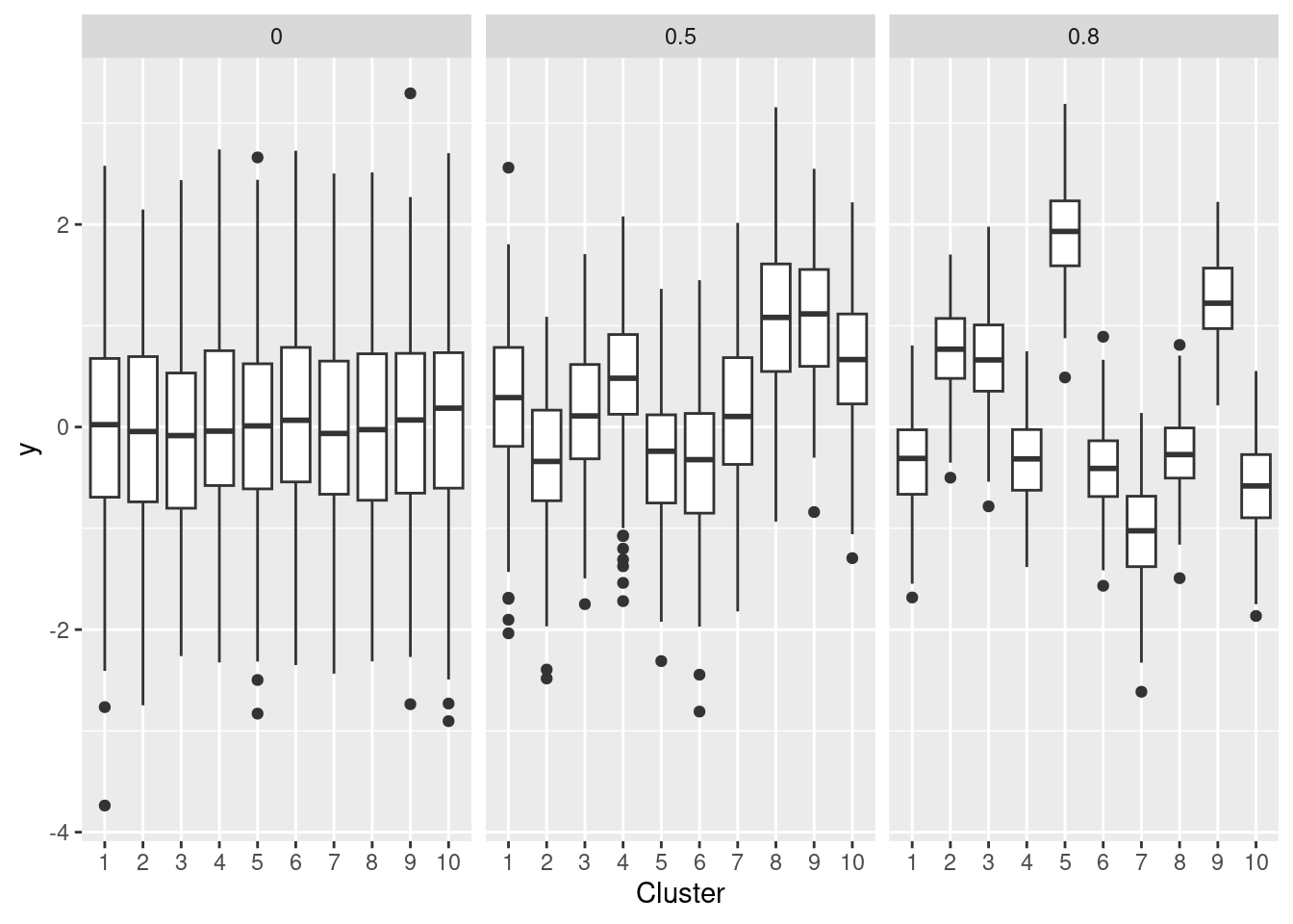
Nei mixed-models è utile capire ed utilizzare l’ICC. Simuliamo dati pre-post con diversi gradi di intraclass correlation (simuliamo più osservazioni di pre-post così è più chiaro il pattern):

library(ggplot2)
library(tidyverse)

icc <- c(0, 0.5, 0.8)
n <- 10
nt <- 100
b0 <- 0
b1 <- 0

sb0 <- sqrt(icc)
s <- sqrt(1 - sb0^2)

dat <- expand.grid(
    id = 1:n,
    x = c(0, 1),
    nt = 1:nt
)

y <- vector(mode = "list", length = length(icc))

for(i in 1:length(y)){
    b0i <- rnorm(n, 0, sb0[i])
    y[[i]] <- rnorm(nrow(dat), with(dat, b0 + b0i[id] + b1 * x), s[i])
}

names(y) <- paste0("y_icc", icc)
dat <- cbind(dat, y)

dat |> 
    pivot_longer(starts_with("y"),
                 names_to = "icc",
                 values_to = "y") |> 
    mutate(icc = parse_number(icc)) |> 
    ggplot(aes(x = factor(id), y = y)) +
    geom_boxplot() +
    facet_wrap(~icc) +
    xlab("Cluster")